

Solutions to exercises
43
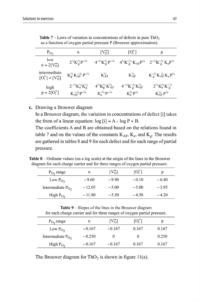
Table 7 – Laws of variation in concentrations of defects in pure ThO 2
as a function of oxygen partial pressure P (Brouwer approximation).
P O 2
n
[V O
••
]
[O′′ i ]
p
low
n = 2[V
••
O ]
2
⅓
K
⅓
g P
−¹⁄6
4
−⅓
K
⅓
g P
−¹⁄6
4
⅓
K
−⅓
g K AF P
¹⁄6
2
−⅓
K
−⅓
g K e P
¹⁄6
intermediate
[O′′ i ] = [V
••
O ]
K
½
g K AF
−¼
P
−¼
K
½
AF
K
½
AF
K
−½
g K AF
¼
K e P
¼
high
p = 2[O′′ i ]
2
−⅓
K
⅓
e K
⅓
g
K AF
−⅓
P
−¹⁄6
4
⅓
K
⅓
g K
⅔
AF
K e
−⅔
P
−¹⁄6
4
−⅓
K
−⅓
g K
⅓
AF
K e
⅔
P
¹⁄6
2
⅓
K e
⅔
K
−⅓
g
K
⅓
AF P
¹⁄6
c. Drawing a Brouwer diagram
In a Brouwer diagram, the variation in concentrations of defect [i] takes
the from of a linear equation: log [i] = A # log P + B.
The coefficients A and B are obtained based on the relations found in
table 7 and on the values of the constants K AF , K e , and K g . The results
are gathered in tables 8 and 9 for each defect and for each range of partial
pressure.
Table 8 – Ordinate values (on a log scale) at the origin of the lines in the Brouwer
diagram for each charge carrier and for three ranges of oxygen partial pressure.
P O 2 range
n
[V
••
O ]
[O′′ i ]
p
Low P O 2
− 9.60
− 9.90
− 0.10
− 6.40
Intermediate P O 2
− 12.05
− 5.00
− 5.00
− 3.95
High P O 2
− 11.80
− 5.50
− 4.50
− 4.20
Table 9 – Slopes of the lines in the Brouwer diagram
for each charge carrier and for three ranges of oxygen partial pressure.
P O 2 range
n
[V
••
O ]
[O′′ i ]
p
Low P O 2
− 0.167
− 0.167
0.167
0.167
Intermediate P O 2
− 0.250
0
0
0.250
High P O 2
− 0.167
− 0.167
0.167
0.167
The Brouwer diagram for ThO 2 is shown in figure 11(a).
43
Table 7 – Laws of variation in concentrations of defects in pure ThO 2
as a function of oxygen partial pressure P (Brouwer approximation).
P O 2
n
[V O
••
]
[O′′ i ]
p
low
n = 2[V
••
O ]
2
⅓
K
⅓
g P
−¹⁄6
4
−⅓
K
⅓
g P
−¹⁄6
4
⅓
K
−⅓
g K AF P
¹⁄6
2
−⅓
K
−⅓
g K e P
¹⁄6
intermediate
[O′′ i ] = [V
••
O ]
K
½
g K AF
−¼
P
−¼
K
½
AF
K
½
AF
K
−½
g K AF
¼
K e P
¼
high
p = 2[O′′ i ]
2
−⅓
K
⅓
e K
⅓
g
K AF
−⅓
P
−¹⁄6
4
⅓
K
⅓
g K
⅔
AF
K e
−⅔
P
−¹⁄6
4
−⅓
K
−⅓
g K
⅓
AF
K e
⅔
P
¹⁄6
2
⅓
K e
⅔
K
−⅓
g
K
⅓
AF P
¹⁄6
c. Drawing a Brouwer diagram
In a Brouwer diagram, the variation in concentrations of defect [i] takes
the from of a linear equation: log [i] = A # log P + B.
The coefficients A and B are obtained based on the relations found in
table 7 and on the values of the constants K AF , K e , and K g . The results
are gathered in tables 8 and 9 for each defect and for each range of partial
pressure.
Table 8 – Ordinate values (on a log scale) at the origin of the lines in the Brouwer
diagram for each charge carrier and for three ranges of oxygen partial pressure.
P O 2 range
n
[V
••
O ]
[O′′ i ]
p
Low P O 2
− 9.60
− 9.90
− 0.10
− 6.40
Intermediate P O 2
− 12.05
− 5.00
− 5.00
− 3.95
High P O 2
− 11.80
− 5.50
− 4.50
− 4.20
Table 9 – Slopes of the lines in the Brouwer diagram
for each charge carrier and for three ranges of oxygen partial pressure.
P O 2 range
n
[V
••
O ]
[O′′ i ]
p
Low P O 2
− 0.167
− 0.167
0.167
0.167
Intermediate P O 2
− 0.250
0
0
0.250
High P O 2
− 0.167
− 0.167
0.167
0.167
The Brouwer diagram for ThO 2 is shown in figure 11(a).