

166
3 – Transport in ionic solids
ij
ij
3W,
ij
3W,,
ij
$X
ij
02
ij
<6=
ij
3W
3W,$X02 <[ <6=3W2 3W,,
Į
ȕ
Ȥ
į
İ
¨(
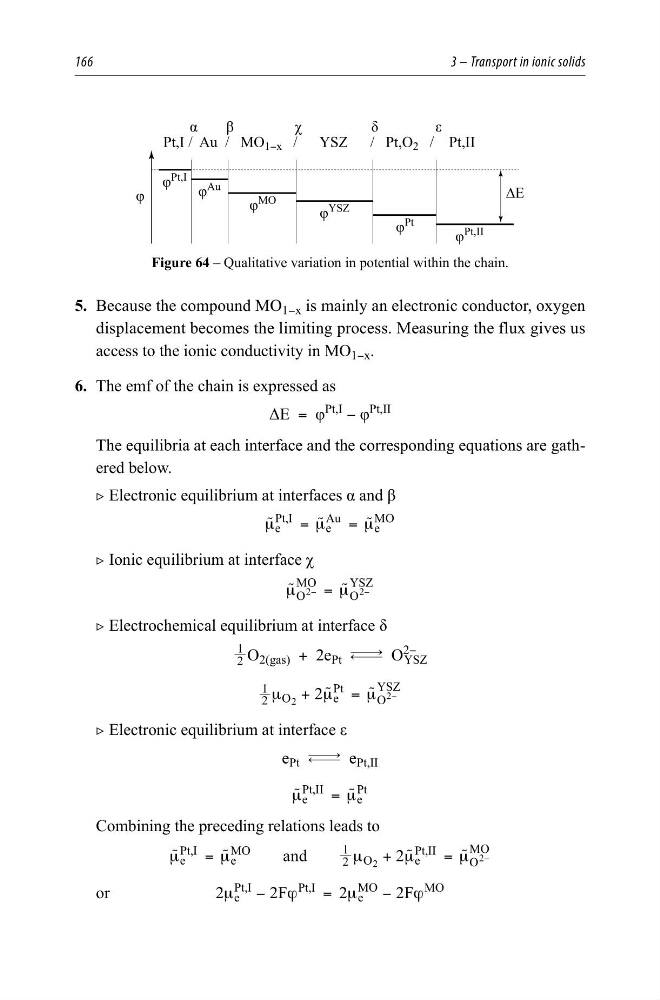
Figure 64 – Qualitative variation in potential within the chain.
5. Because the compound MO 1−x is mainly an electronic conductor, oxygen
displacement becomes the limiting process. Measuring the flux gives us
access to the ionic conductivity in MO 1−x .
6. The emf of the chain is expressed as
ΔE = φ
Pt,I − φ
Pt,II
The equilibria at each interface and the corresponding equations are gathered below.
2 Electronic equilibrium at interfaces α and β
e
Pt,I
e
Au
e
MO
μ
μ
μ
=
=
u
u
u
2 Ionic equilibrium at interface χ
O
MO
O
YSZ
2
2
μ
μ
=
−
−
u
u
2 Electrochemical equilibrium at interface δ
2
1
O 2(gas) + 2e Pt m O
2−
YSZ
2
2
1 O
e
Pt
O
YSZ
2
2
μ
μ
μ
+
=
−
u
u
2 Electronic equilibrium at interface ε
e Pt m e Pt,II
e
Pt,II
e
Pt
μ
μ
=
u
u
Combining the preceding relations leads to
and
2
e
Pt,I
e
MO
2
1 O
e
Pt,II
O
MO
2
2
μ
μ
μ
μ
μ
=
+
=
−
u
u
u
u
or
2
2F
2
2F
e
Pt,I
Pt,I
e
MO
MO
μ
ϕ
μ
ϕ
−
=
−
3 – Transport in ionic solids
ij
ij
3W,
ij
3W,,
ij
$X
ij
02
ij
<6=
ij
3W
3W,$X02 <[ <6=3W2 3W,,
Į
ȕ
Ȥ
į
İ
¨(
Figure 64 – Qualitative variation in potential within the chain.
5. Because the compound MO 1−x is mainly an electronic conductor, oxygen
displacement becomes the limiting process. Measuring the flux gives us
access to the ionic conductivity in MO 1−x .
6. The emf of the chain is expressed as
ΔE = φ
Pt,I − φ
Pt,II
The equilibria at each interface and the corresponding equations are gathered below.
2 Electronic equilibrium at interfaces α and β
e
Pt,I
e
Au
e
MO
μ
μ
μ
=
=
u
u
u
2 Ionic equilibrium at interface χ
O
MO
O
YSZ
2
2
μ
μ
=
−
−
u
u
2 Electrochemical equilibrium at interface δ
2
1
O 2(gas) + 2e Pt m O
2−
YSZ
2
2
1 O
e
Pt
O
YSZ
2
2
μ
μ
μ
+
=
−
u
u
2 Electronic equilibrium at interface ε
e Pt m e Pt,II
e
Pt,II
e
Pt
μ
μ
=
u
u
Combining the preceding relations leads to
and
2
e
Pt,I
e
MO
2
1 O
e
Pt,II
O
MO
2
2
μ
μ
μ
μ
μ
=
+
=
−
u
u
u
u
or
2
2F
2
2F
e
Pt,I
Pt,I
e
MO
MO
μ
ϕ
μ
ϕ
−
=
−