

162
3 – Transport in ionic solids
We find good agreement between the experimental points and the theoretical models.
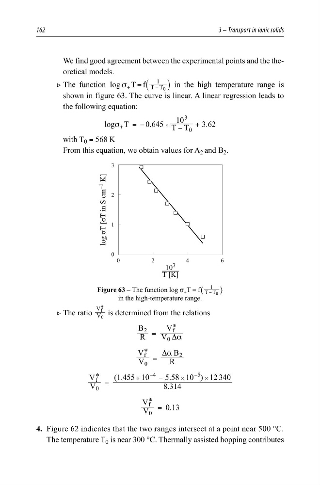
2 The function log T f T T
1
0
σ =
+
−
`
j in the high temperature range is
shown in figure 63. The curve is linear. A linear regression leads to
the following equation:
log T
0.645 T T
10
3.62
0
3
σ
= −
−
+
+
#
with T 0 = 568 K
From this equation, we obtain values for A 2 and B 2 .
—
7>.@
ORJı7>ı7LQ6FP
<
.@
Figure 63 – The function log σ + T = f T T
1
−
^
h
in the high-temperature range.
2 The ratio V
V f
0
* is determined from the relations
R
B
V
V
2
0
f
α
Δ
=
*
V
V
R
B
0
f
2
α
Δ
=
*
.
( .
.
)
V
V
8 314
1 455 10
5 58 10
12 340
f
0
4
5
#
#
=
−
−
− #
*
.
V
V
0 13
f
0
=
*
4. Figure 62 indicates that the two ranges intersect at a point near 500 °C.
The temperature T 0 is near 300 °C. Thermally assisted hopping contributes
3 – Transport in ionic solids
We find good agreement between the experimental points and the theoretical models.
2 The function log T f T T
1
0
σ =
+
−
`
j in the high temperature range is
shown in figure 63. The curve is linear. A linear regression leads to
the following equation:
log T
0.645 T T
10
3.62
0
3
σ
= −
−
+
+
#
with T 0 = 568 K
From this equation, we obtain values for A 2 and B 2 .
—
7>.@
ORJı7>ı7LQ6FP
<
.@
Figure 63 – The function log σ + T = f T T
1
−
^
h
in the high-temperature range.
2 The ratio V
V f
0
* is determined from the relations
R
B
V
V
2
0
f
α
Δ
=
*
V
V
R
B
0
f
2
α
Δ
=
*
.
( .
.
)
V
V
8 314
1 455 10
5 58 10
12 340
f
0
4
5
#
#
=
−
−
− #
*
.
V
V
0 13
f
0
=
*
4. Figure 62 indicates that the two ranges intersect at a point near 500 °C.
The temperature T 0 is near 300 °C. Thermally assisted hopping contributes