

100
3 – Transport in ionic solids
3.3 – Basic description of Wagner theory
The goal is to express the potential difference ΔU between the terminals of a
mixed-conduction ionic crystal subjected to a chemical potential gradient from
one of its constituents. For this, we consider the following electrochemical chain:
X 2 (P a ), M / AX / M, X 2 (P b )
which involves a mixed conductor (ionic + electronic) AX, two identical metallic electrodes M, and the different partial pressures P a and P b of the gas X 2 .
The following hypotheses are considered:
2 local equilibrium at each point in the chain,
2 electroneutrality at each point,
2 steady state,
2 negligible overvoltage at the electrodes.
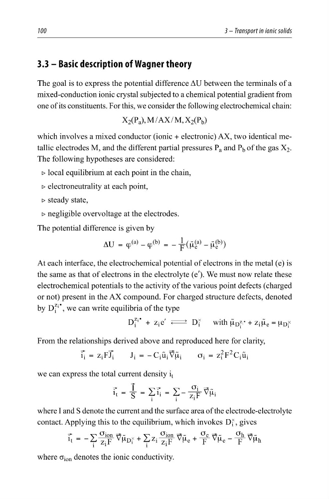
The potential difference is given by
U
F
1
(a)
(b)
e
(a)
e
(b)
ϕ
ϕ
μ
μ
Δ =
−
= −
−
u
u
^
h
At each interface, the electrochemical potential of electrons in the metal (e) is
the same as that of electrons in the electrolyte (e ′ ). We must now relate these
electrochemical potentials to the activity of the various point defects (charged
or not) present in the AX compound. For charged structure defects, denoted
by D i
z •
i
, we can write equilibria of the type
D
z e
i
z
i
•
i
+
l m D i
#
with
z
D
i e
D
i
z •
i
i
μ
μ μ
+
= #
u
u
From the relationships derived above and reproduced here for clarity,
i
z FJ
J
C u
zF C u
i
i i
i
i i
i
i
i
2 2 i i
dμ
σ
=
=−
=
u u
u
we can express the total current density i t
i
S
I
i
z F
t
i
i
i
i
i
i
d
σ
μ
=
=
= −
u
/
/
where I and S denote the current and the surface area of the electrode-electrolyte
contact. Applying this to the equilibrium, which invokes D i
#
, gives
i
z F
z z F
F
F
t
i
ion
i
D
i i
ion
i
e
e
e
h
h
i
d
d
d
d
σ
μ
σ
μ
σ μ
σ μ
= −
+
+
−
#
u
u
u
u
/
/
where σ ion denotes the ionic conductivity.
3 – Transport in ionic solids
3.3 – Basic description of Wagner theory
The goal is to express the potential difference ΔU between the terminals of a
mixed-conduction ionic crystal subjected to a chemical potential gradient from
one of its constituents. For this, we consider the following electrochemical chain:
X 2 (P a ), M / AX / M, X 2 (P b )
which involves a mixed conductor (ionic + electronic) AX, two identical metallic electrodes M, and the different partial pressures P a and P b of the gas X 2 .
The following hypotheses are considered:
2 local equilibrium at each point in the chain,
2 electroneutrality at each point,
2 steady state,
2 negligible overvoltage at the electrodes.
The potential difference is given by
U
F
1
(a)
(b)
e
(a)
e
(b)
ϕ
ϕ
μ
μ
Δ =
−
= −
−
u
u
^
h
At each interface, the electrochemical potential of electrons in the metal (e) is
the same as that of electrons in the electrolyte (e ′ ). We must now relate these
electrochemical potentials to the activity of the various point defects (charged
or not) present in the AX compound. For charged structure defects, denoted
by D i
z •
i
, we can write equilibria of the type
D
z e
i
z
i
•
i
+
l m D i
#
with
z
D
i e
D
i
z •
i
i
μ
μ μ
+
= #
u
u
From the relationships derived above and reproduced here for clarity,
i
z FJ
J
C u
zF C u
i
i i
i
i i
i
i
i
2 2 i i
dμ
σ
=
=−
=
u u
u
we can express the total current density i t
i
S
I
i
z F
t
i
i
i
i
i
i
d
σ
μ
=
=
= −
u
/
/
where I and S denote the current and the surface area of the electrode-electrolyte
contact. Applying this to the equilibrium, which invokes D i
#
, gives
i
z F
z z F
F
F
t
i
ion
i
D
i i
ion
i
e
e
e
h
h
i
d
d
d
d
σ
μ
σ
μ
σ μ
σ μ
= −
+
+
−
#
u
u
u
u
/
/
where σ ion denotes the ionic conductivity.