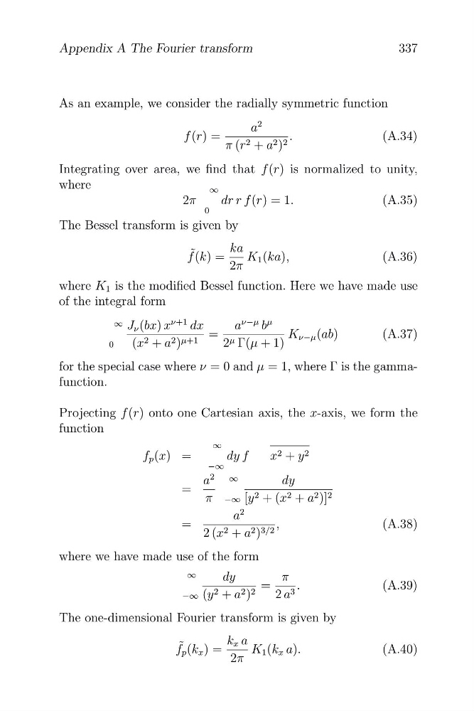
As an example, we consider the radially symmetric function
2
a
f (r) =
.
(A.34)
π (r 2 + a 2 ) 2
Integrating over area, we find that f (r) is normalized to unity,
where
∞
2π
dr r f (r) = 1.
(A.35)
0
The Bessel transform is given by
f ˜ (k) =
ka
2π
K 1 (ka),
(A.36)
where K 1 is the modified Bessel function. Here we have made use
of the integral form
∞
ν+1 dx
ν−µ b
µ
J ν (bx) x
a
=
K ν−µ (ab)
(A.37)
2 + a 2 ) µ+1
0
(x
2 µ Γ(µ + 1)
for the special case where ν = 0 and µ = 1, where Γ is the gammafunction.
Projecting f (r) onto one Cartesian axis, the x-axis, we form the
2 (x 2 + a 2 ) 3/2
function
∞
f p (x) =
−∞
dy f
x 2 + y 2
a
2
∞
dy
= π −∞ [y 2 + (x 2 + a 2 )] 2
a
2
=
,
(A.38)
where we have made use of the form

∞
dy
π
=
.
(A.39)
2 + a 2 ) 2
3
−∞ (y
2 a
The one-dimensional Fourier transform is given by
f ˜ p (k x ) =
k x a K 1 (k x a).
(A.40)
2π
337
Appendix A The Fourier transform