

space (x, y). This will turn out to be very useful in reducing the
number of degrees of freedom in problems of multiple variables.
In particular, it greatly simplifies the problem of the stochastic
Coulomb interaction in a charged particle beam.
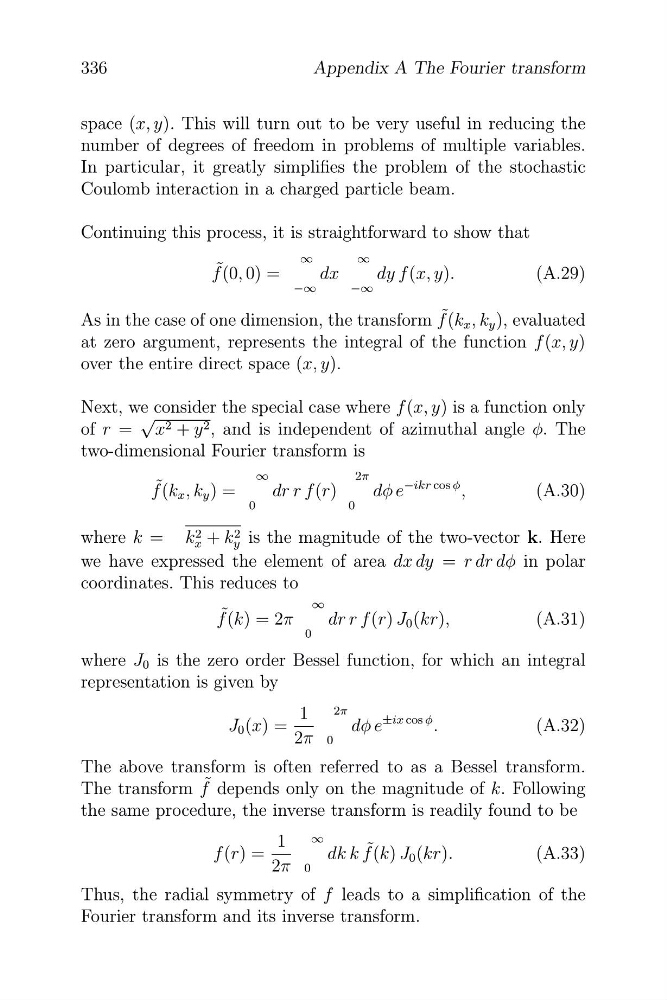
Continuing this process, it is straightforward to show that
∞
∞
f ˜ (0, 0) =
dx
dy f (x, y).
(A.29)
−∞
−∞
As in the case of one dimension, the transform f ˜ (k x , k y ), evaluated
at zero argument, represents the integral of the function f (x, y)
over the entire direct space (x, y).
Next, we consider the special case where f (x, y) is a function only
√
of r = x 2 + y 2 , and is independent of azimuthal angle φ. The
two-dimensional Fourier transform is
∞
2π
f ˜ (k x , k y ) =
dr r f (r)
dφ e
−ikr cos φ ,
(A.30)
0
0
where k = k x
2 + k y
2 is the magnitude of the two-vector k. Here
we have expressed the element of area dx dy = r dr dφ in polar
coordinates. This reduces to
f ˜ (k) = 2π
∞
dr r f (r) J 0 (kr),
(A.31)
0
where J 0 is the zero order Bessel function, for which an integral
representation is given by
2π
J 0 (x) =
1
dφ e
±ix cos φ .
(A.32)
2π 0
The above transform is often referred to as a Bessel transform.
The transform f ˜ depends only on the magnitude of k. Following
the same procedure, the inverse transform is readily found to be
f (r) =
1 ∞
dk k f ˜ (k) J 0 (kr).
(A.33)
2π 0
Thus, the radial symmetry of f leads to a simplification of the
Fourier transform and its inverse transform.
336
Appendix A The Fourier transform
number of degrees of freedom in problems of multiple variables.
In particular, it greatly simplifies the problem of the stochastic
Coulomb interaction in a charged particle beam.
Continuing this process, it is straightforward to show that
∞
∞
f ˜ (0, 0) =
dx
dy f (x, y).
(A.29)
−∞
−∞
As in the case of one dimension, the transform f ˜ (k x , k y ), evaluated
at zero argument, represents the integral of the function f (x, y)
over the entire direct space (x, y).
Next, we consider the special case where f (x, y) is a function only
√
of r = x 2 + y 2 , and is independent of azimuthal angle φ. The
two-dimensional Fourier transform is
∞
2π
f ˜ (k x , k y ) =
dr r f (r)
dφ e
−ikr cos φ ,
(A.30)
0
0
where k = k x
2 + k y
2 is the magnitude of the two-vector k. Here
we have expressed the element of area dx dy = r dr dφ in polar
coordinates. This reduces to
f ˜ (k) = 2π
∞
dr r f (r) J 0 (kr),
(A.31)
0
where J 0 is the zero order Bessel function, for which an integral
representation is given by
2π
J 0 (x) =
1
dφ e
±ix cos φ .
(A.32)
2π 0
The above transform is often referred to as a Bessel transform.
The transform f ˜ depends only on the magnitude of k. Following
the same procedure, the inverse transform is readily found to be
f (r) =
1 ∞
dk k f ˜ (k) J 0 (kr).
(A.33)
2π 0
Thus, the radial symmetry of f leads to a simplification of the
Fourier transform and its inverse transform.
336
Appendix A The Fourier transform