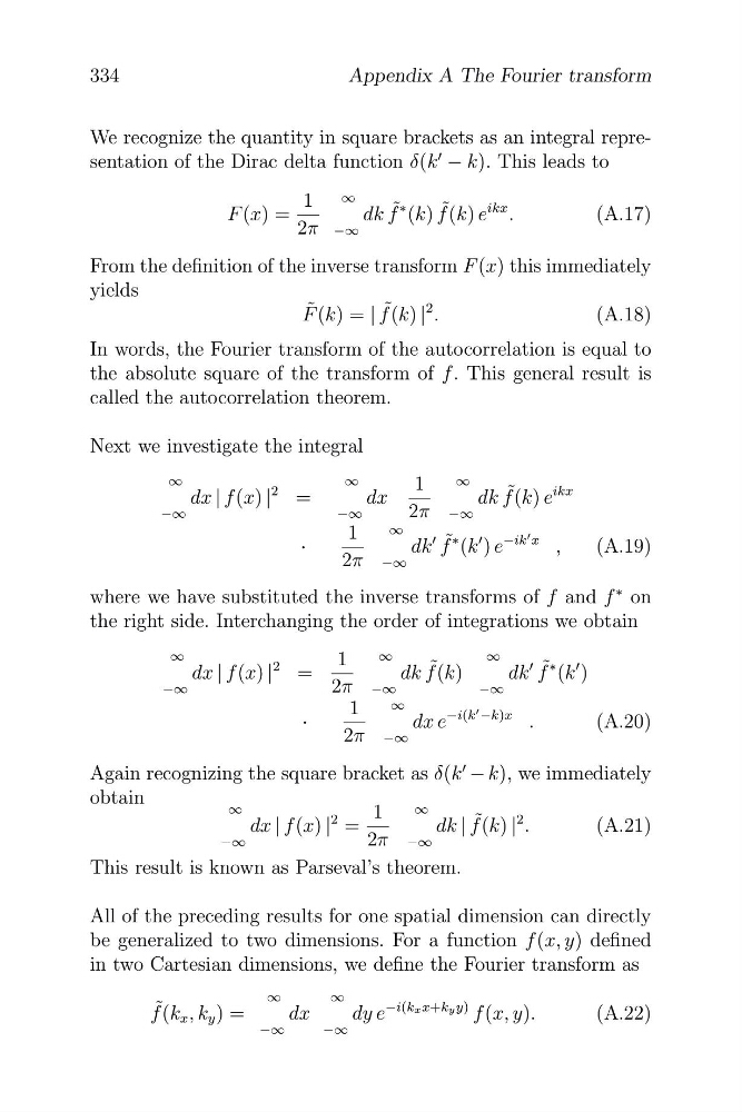
�
�
�
�
�
�
We recognize the quantity in square brackets as an integral representation of the Dirac delta function δ(k
� − k). This leads to
F (x) =
1 ∞
dk f ˜ ∗ (k) f ˜ (k) e
ikx .
(A.17)
2π −∞
From the definition of the inverse transform F (x) this immediately
yields
˜
F (k) = | f ˜ (k) |
2 .
(A.18)
In words, the Fourier transform of the autocorrelation is equal to
the absolute square of the transform of f . This general result is
called the autocorrelation theorem.
Next we investigate the integral
∞
∞
∞
1
dx | f (x) |
2 =
dx
dk f ˜ (k) e
ikx
−∞
−∞
2π −∞
−ik � x
·
1
∞
dk
� f ˜ ∗ (k
� ) e
,
(A.19)
2π −∞
where we have substituted the inverse transforms of f and f
∗ on
the right side. Interchanging the order of integrations we obtain
∞
∞
∞
1
dx | f (x) |
2 =
dk f ˜ (k)
dk
� f ˜ ∗ (k
� )
−∞
2π −∞
−∞

1

·
∞
dx e
−i(k � −k)x .
(A.20)
2π −∞
Again recognizing the square bracket as δ(k
� − k), we immediately
obtain
∞
∞
1
dx | f (x) |
2 =
dk | f ˜ (k) |
2 .
(A.21)
−∞
2π −∞
This result is known as Parseval’s theorem.
All of the preceding results for one spatial dimension can directly
be generalized to two dimensions. For a function f (x, y) defined
in two Cartesian dimensions, we define the Fourier transform as
f ˜ (k x , k y ) =
∞
dx
∞
dy e
−i(kxx+ky y) f (x, y).
(A.22)
−∞
−∞
334
Appendix A The Fourier transform