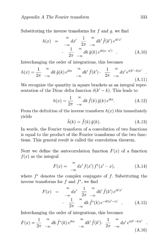
�
�
�
�
�
�
�
�
�
�
�
�
Substituting the inverse transforms for f and g, we find
1
ik � x �
h(x) =
∞
dx
�
∞
dk
� f ˜ (k
� ) e
−∞
2π −∞
1 ∞
� )
ik(x−x
·
dk g ˜(k) e
.
(A.10)
2π −∞
Interchanging the order of integrations, this becomes
∞
∞
∞
1
ikx
f ˜ (k
� ) ·
1
i(k � −k)x �
h(x) =
dk g ˜(k) e
dk
�
dx
� e
.
2π −∞
−∞
2π −∞
(A.11)
We recognize the quantity in square brackets as an integral representation of the Dirac delta function δ(k
� − k). This leads to
h(x) =
1 ∞
dk f ˜ (k) ˜
g(k) e
ikx .
(A.12)
2π −∞
From the definition of the inverse transform h(x) this immediately
yields
h ˜ (k) = f ˜ (k) ˜
g(k).
(A.13)
In words, the Fourier transform of a convolution of two functions
is equal to the product of the Fourier transforms of the two functions. This general result is called the convolution theorem.
Next we define the autocorrelation function F (x) of a function
f (x) as the integral
F (x) =
∞
dx
� f (x
� ) f
∗ (x
� − x),
(A.14)
−∞
where f
∗ denotes the complex conjugate of f . Substituting the
inverse transforms for f and f
∗ , we find
1
�
F (x) =
∞
dx
�
∞
dk
� f ˜ (k
� ) e
ik � x
−∞
2π −∞
−ik(x
·
1 ∞
dk f ˜ ∗ (k) e
� −x) .
(A.15)
2π −∞
Interchanging the order of integrations, this becomes
∞
∞
∞
1
1
�
ikx
i(k � −k)x
F (x) =
dk f ˜ ∗ (k) e
dk
� f ˜ (k
� )·
dx
� e
.
2π −∞
−∞
2π −∞
(A.16)
333
Appendix A The Fourier transform