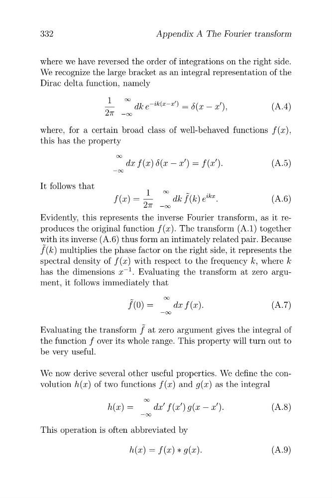
where we have reversed the order of integrations on the right side.
We recognize the large bracket as an integral representation of the
Dirac delta function, namely
1 ∞
� )
dk e
−ik(x−x = δ(x − x
� ),
(A.4)
2π −∞
where, for a certain broad class of well-behaved functions f (x),
this has the property
∞
dx f (x) δ(x − x
� ) = f (x
� ).
(A.5)
−∞
It follows that
f (x) =
1 ∞
dk f ˜ (k) e
ikx .
(A.6)
2π −∞
Evidently, this represents the inverse Fourier transform, as it reproduces the original function f (x). The transform (A.1) together
with its inverse (A.6) thus form an intimately related pair. Because
f ˜ (k) multiplies the phase factor on the right side, it represents the
spectral density of f (x) with respect to the frequency k, where k
has the dimensions x
−1 . Evaluating the transform at zero argument, it follows immediately that
f ˜ (0) =
∞
dx f (x).
(A.7)
−∞
Evaluating the transform f ˜ at zero argument gives the integral of
the function f over its whole range. This property will turn out to
be very useful.
We now derive several other useful properties. We define the convolution h(x) of two functions f (x) and g(x) as the integral
h(x) =
∞
dx
� f (x
� ) g(x − x
� ).
(A.8)
−∞
This operation is often abbreviated by

h(x) = f (x) ∗ g(x).
(A.9)

332
Appendix A The Fourier transform