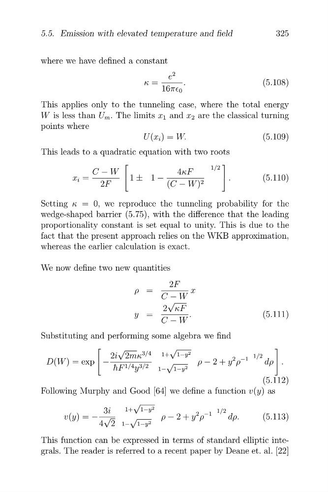
�
�
where we have defined a constant
2
e
κ =
.
(5.108)
16πf 0
This applies only to the tunneling case, where the total energy
W is less than U m . The limits x 1 and x 2 are the classical turning
points where
U (x i ) = W.
(5.109)
This leads to a quadratic equation with two roots
⎡
⎤
1/2
C − W
4κF
x i =
⎣ 1 ± 1 −
⎦ .
(5.110)
2F
(C − W ) 2
Setting κ = 0, we reproduce the tunneling probability for the
wedge-shaped barrier (5.75), with the difference that the leading
proportionality constant is set equal to unity. This is due to the
fact that the present approach relies on the WKB approximation,
whereas the earlier calculation is exact.
We now define two new quantities
2F
ρ =
x
C − W
√
2 κF
y =
.
(5.111)
C − W
Substituting and performing some algebra we find
⎡
⎤
√
√
1+ 1−y 2
2i 2mκ
3/4
1/2
D(W ) = exp ⎣ −
3/2
√
ρ − 2 + y
2 ρ
−1
dρ ⎦ .
¯
y
1− 1−y 2
hF 1/4
(5.112)
Following Murphy and Good [64] we define a function v(y) as
√
3i
1+ 1−y 2
1/2
2 ρ
−1
v(y) = − √
√
ρ − 2 + y
dρ.
(5.113)
4 2 1− 1−y 2
This function can be expressed in terms of standard elliptic integrals. The reader is referred to a recent paper by Deane et. al. [22]
325
5.5. Emission with elevated temperature and field