

�
�
�
�
�
�
321
5.5. Emission with elevated temperature and field
We choose the positive root without loss of generality.
All relevant information is contained in the wave function u(x).
We assume without loss of generality that the wave function can
be expressed as
i
u(x) = exp
S(x) ,
(5.86)
h ¯
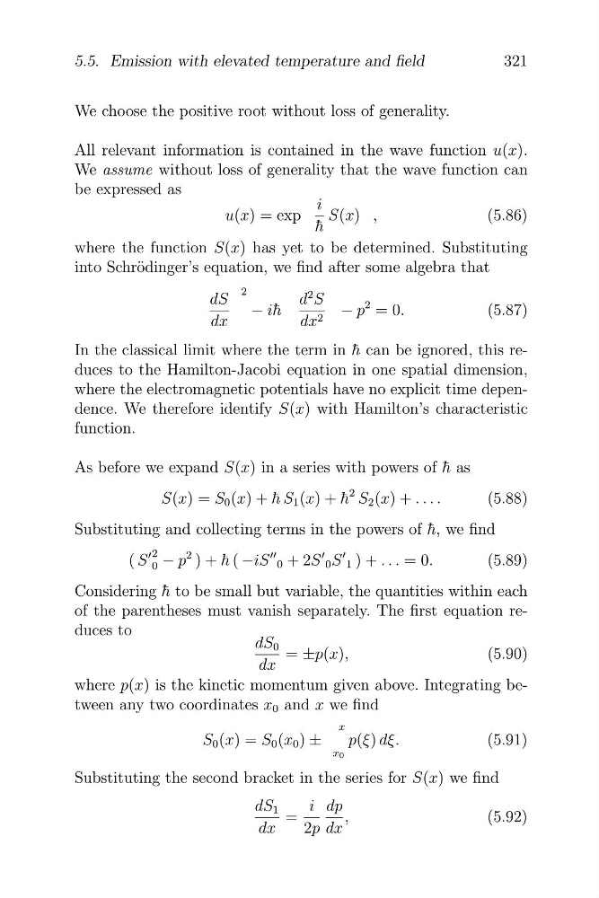
where the function S(x) has yet to be determined. Substituting
into Schr¨ odinger’s equation, we find after some algebra that
dS
2
d
2 S
− ih ¯
− p
2 = 0.
(5.87)
dx
dx 2
In the classical limit where the term in ¯
h can be ignored, this reduces to the Hamilton-Jacobi equation in one spatial dimension,
where the electromagnetic potentials have no explicit time dependence. We therefore identify S(x) with Hamilton’s characteristic
function.
As before we expand S(x) in a series with powers of ¯
h as
S(x) = S 0 (x) + ¯
h S 1 (x) + ¯
h
2 S 2 (x) + . . . .
(5.88)
Substituting and collecting terms in the powers of ¯
h, we find
( S
� 2
0 − p
2 ) + ¯
h ( −iS
��
0 + 2S
�
0 S
�
1 ) + . . . = 0.
(5.89)
Considering ¯
h to be small but variable, the quantities within each
of the parentheses must vanish separately. The first equation reduces to
dS 0 = ±p(x),
(5.90)
dx
where p(x) is the kinetic momentum given above. Integrating between any two coordinates x 0 and x we find
x
S 0 (x) = S 0 (x 0 ) ±
p(ξ) dξ.
(5.91)
x 0
Substituting the second bracket in the series for S(x) we find
dS 1
i dp
=
,
(5.92)
dx
2p dx
�
�
�
�
�
321
5.5. Emission with elevated temperature and field
We choose the positive root without loss of generality.
All relevant information is contained in the wave function u(x).
We assume without loss of generality that the wave function can
be expressed as
i
u(x) = exp
S(x) ,
(5.86)
h ¯
where the function S(x) has yet to be determined. Substituting
into Schr¨ odinger’s equation, we find after some algebra that
dS
2
d
2 S
− ih ¯
− p
2 = 0.
(5.87)
dx
dx 2
In the classical limit where the term in ¯
h can be ignored, this reduces to the Hamilton-Jacobi equation in one spatial dimension,
where the electromagnetic potentials have no explicit time dependence. We therefore identify S(x) with Hamilton’s characteristic
function.
As before we expand S(x) in a series with powers of ¯
h as
S(x) = S 0 (x) + ¯
h S 1 (x) + ¯
h
2 S 2 (x) + . . . .
(5.88)
Substituting and collecting terms in the powers of ¯
h, we find
( S
� 2
0 − p
2 ) + ¯
h ( −iS
��
0 + 2S
�
0 S
�
1 ) + . . . = 0.
(5.89)
Considering ¯
h to be small but variable, the quantities within each
of the parentheses must vanish separately. The first equation reduces to
dS 0 = ±p(x),
(5.90)
dx
where p(x) is the kinetic momentum given above. Integrating between any two coordinates x 0 and x we find
x
S 0 (x) = S 0 (x 0 ) ±
p(ξ) dξ.
(5.91)
x 0
Substituting the second bracket in the series for S(x) we find
dS 1
i dp
=
,
(5.92)
dx
2p dx