

�
�
p(x 0 )
where we have made use of
S
��
0 (x) = ±p
� (x).
(5.93)
Integrating between the limits x 0 and x we find
S 1 (x) = S 1 (x 0 ) + i ln
p(x)
1/2
.
(5.94)
h
2
Substituting above, and ignoring terms in ¯ and higher, we find
the approximate solution for the wave function u(x) as
1/2
x
p(x 0 )
i
u(x) ≈ u(x 0 )
exp ±
p(ξ) dξ .
(5.95)
p(x)
h ¯ x 0
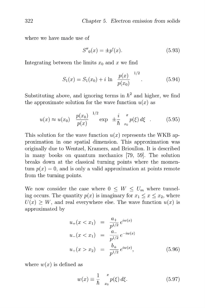
This solution for the wave function u(x) represents the WKB approximation in one spatial dimension. This approximation was
originally due to Wentzel, Kramers, and Brioullon. It is described
in many books on quantum mechanics [79, 59]. The solution
breaks down at the classical turning points where the momentum p(x) = 0, and is only a valid approximation at points remote
from the turning points.
We now consider the case where 0 ≤ W ≤ U m where tunneling occurs. The quantity p(x) is imaginary for x 1 ≤ x ≤ x 2 , where
U (x) ≥ W , and real everywhere else. The wave function u(x) is
approximated by
a + iw(x)
u + (x < x 1 ) =
e
1/2
p
a − −iw(x)
u − (x < x 1 ) =
e
1/2
p
b + iw(x)
u + (x > x 2 ) =
e
,
(5.96)
p 1/2
where w(x) is defined as
1 x
w(x) ≡ ¯
h x 0
p(ξ) dξ.
(5.97)
322
Chapter 5. Electron emission from solids
�
p(x 0 )
where we have made use of
S
��
0 (x) = ±p
� (x).
(5.93)
Integrating between the limits x 0 and x we find
S 1 (x) = S 1 (x 0 ) + i ln
p(x)
1/2
.
(5.94)
h
2
Substituting above, and ignoring terms in ¯ and higher, we find
the approximate solution for the wave function u(x) as
1/2
x
p(x 0 )
i
u(x) ≈ u(x 0 )
exp ±
p(ξ) dξ .
(5.95)
p(x)
h ¯ x 0
This solution for the wave function u(x) represents the WKB approximation in one spatial dimension. This approximation was
originally due to Wentzel, Kramers, and Brioullon. It is described
in many books on quantum mechanics [79, 59]. The solution
breaks down at the classical turning points where the momentum p(x) = 0, and is only a valid approximation at points remote
from the turning points.
We now consider the case where 0 ≤ W ≤ U m where tunneling occurs. The quantity p(x) is imaginary for x 1 ≤ x ≤ x 2 , where
U (x) ≥ W , and real everywhere else. The wave function u(x) is
approximated by
a + iw(x)
u + (x < x 1 ) =
e
1/2
p
a − −iw(x)
u − (x < x 1 ) =
e
1/2
p
b + iw(x)
u + (x > x 2 ) =
e
,
(5.96)
p 1/2
where w(x) is defined as
1 x
w(x) ≡ ¯
h x 0
p(ξ) dξ.
(5.97)
322
Chapter 5. Electron emission from solids