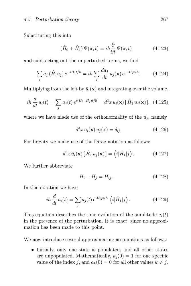
Substituting this into
( ˆ
H 0 + ˆ
H 1 ) Ψ(x, t) = i¯ h
∂
∂t
Ψ(x, t)
and subtracting out the unperturbed terms, we find
4
j
a j ( ˆ
H 1 u j ) e
−iH j t/¯ h = i¯ h
4
j
da j
dt
u j (x) e
−iH j t/¯ h .
(4.123)
(4.124)
Multiplying from the left by ¯
u i (x) and integrating over the volume,
4
d
i(H i −H j )t/¯ h
ih ¯ a i (t) =
a j (t) e
d
3 x u ¯ i (x) [ H ˆ 1 u j (x) ], (4.125)
dt
j
where we have made use of the orthonormality of the u j , namely
d
3 x ¯
u i (x) u j (x) = δ ij .
(4.126)
For brevity we make use of the Dirac notation as
d
3 x ¯
u i (x) [ ˆ
H 1 u j (x) ] = i| ˆ
H 1 |j
We further abbreviate
follo
.
ws:
(4.127)
H i − H j = H ij .
(4.128)
In this notation we have
4
d
iH ij t/¯ h
ih ¯ a i (t) =
a j (t) e
i|H ˆ 1 |j .
(4.129)
dt
j
This equation describes the time evolution of the amplitude a i (t)
in the presence of the perturbation. It is exact, since no approximation has been made to this point.
We now introduce several approximating assumptions as follows:
• Initially, only one state is populated, and all other states
are unpopulated. Mathematically, a j (0) = 1 for one specific
value of the index j, and a k (0) = 0 for all other values k = j.
4.5. Perturbation theory
267
�