

266
Chapter 4. Particle scattering
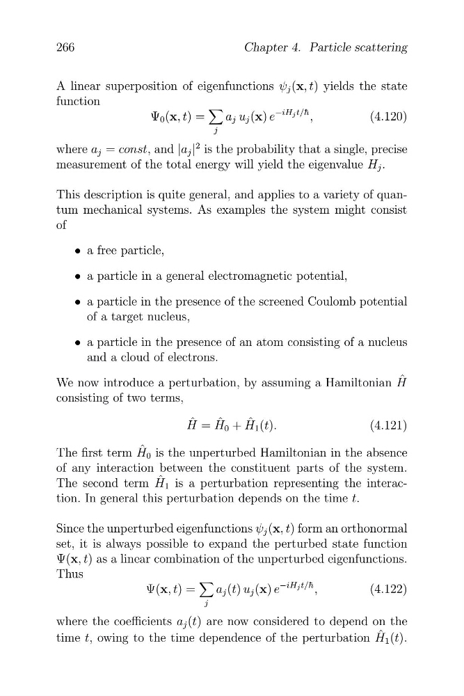
A linear superposition of eigenfunctions ψ j (x, t) yields the state
function
4
−iH j t/¯ h
Ψ 0 (x, t) =
a j u j (x) e
,
(4.120)
j
where a j = const, and |a j |
2 is the probability that a single, precise
measurement of the total energy will yield the eigenvalue H j .
This description is quite general, and applies to a variety of quantum mechanical systems. As examples the system might consist
of
• a free particle,
• a particle in a general electromagnetic potential,
• a particle in the presence of the screened Coulomb potential
of a target nucleus,
• a particle in the presence of an atom consisting of a nucleus
and a cloud of electrons.
ˆ
We now introduce a perturbation, by assuming a Hamiltonian H
consisting of two terms,
H ˆ = H ˆ 0 + H ˆ 1 (t).
(4.121)
ˆ
The first term H 0 is the unperturbed Hamiltonian in the absence
of any interaction between the constituent parts of the system.
ˆ
The second term H 1 is a perturbation representing the interaction. In general this perturbation depends on the time t.
Since the unperturbed eigenfunctions ψ j (x, t) form an orthonormal
set, it is always possible to expand the perturbed state function
Ψ(x, t) as a linear combination of the unperturbed eigenfunctions.
Thus
4
−iH j t/¯ h
Ψ(x, t) =
a j (t) u j (x) e
,
(4.122)
j
where the coefficients a j (t) are now considered to depend on the
ˆ
time t, owing to the time dependence of the perturbation H 1 (t).
Chapter 4. Particle scattering
A linear superposition of eigenfunctions ψ j (x, t) yields the state
function
4
−iH j t/¯ h
Ψ 0 (x, t) =
a j u j (x) e
,
(4.120)
j
where a j = const, and |a j |
2 is the probability that a single, precise
measurement of the total energy will yield the eigenvalue H j .
This description is quite general, and applies to a variety of quantum mechanical systems. As examples the system might consist
of
• a free particle,
• a particle in a general electromagnetic potential,
• a particle in the presence of the screened Coulomb potential
of a target nucleus,
• a particle in the presence of an atom consisting of a nucleus
and a cloud of electrons.
ˆ
We now introduce a perturbation, by assuming a Hamiltonian H
consisting of two terms,
H ˆ = H ˆ 0 + H ˆ 1 (t).
(4.121)
ˆ
The first term H 0 is the unperturbed Hamiltonian in the absence
of any interaction between the constituent parts of the system.
ˆ
The second term H 1 is a perturbation representing the interaction. In general this perturbation depends on the time t.
Since the unperturbed eigenfunctions ψ j (x, t) form an orthonormal
set, it is always possible to expand the perturbed state function
Ψ(x, t) as a linear combination of the unperturbed eigenfunctions.
Thus
4
−iH j t/¯ h
Ψ(x, t) =
a j (t) u j (x) e
,
(4.122)
j
where the coefficients a j (t) are now considered to depend on the
ˆ
time t, owing to the time dependence of the perturbation H 1 (t).