

219
3.3. Diffraction
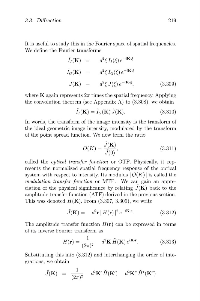
It is useful to study this in the Fourier space of spatial frequencies.
We define the Fourier transforms
−iK·ξ
I ˜ I (K) =
d
2 ξ I I (ξ) e
−iK·ξ
I ˜ G (K) =
d
2 ξ I G (ξ) e
−iK·ξ
J ˜ (K) =
d
2 ξ J(ξ) e
,
(3.309)
where K again represents 2π times the spatial frequency. Applying
the convolution theorem (see Appendix A) to (3.308), we obtain
I ˜ I (K) = I ˜ G (K) J ˜ (K).
(3.310)
In words, the transform of the image intensity is the transform of
the ideal geometric image intensity, modulated by the transform
of the point spread function. We now form the ratio
˜
J(K)
O(K) =
,
(3.311)
˜
J(0)
called the optical transfer function or OTF. Physically, it represents the normalized spatial frequency response of the optical
system with respect to intensity. Its modulus | O(K) | is called the
modulation transfer function or MTF. We can gain an appre˜
ciation of the physical significance by relating J(K) back to the
amplitude transfer function (ATF) derived in the previous section.
˜
This was denoted H(K). From (3.307, 3.309), we write
˜
d
2
−iK·r
J(K) =
r | H(r) |
2 e
.
(3.312)
The amplitude transfer function H(r) can be expressed in terms
of its inverse Fourier transform as
H(r) =
1
d
2 K H ˜ (K) e
iK·r .
(3.313)
(2π) 2
Substituting this into (3.312) and interchanging the order of integrations, we obtain
˜
1
d
2 K
� ˜
d
2 K
�� H ˜ ∗ (K
�� )
J(K) =
H(K
� )
(2π) 2
3.3. Diffraction
It is useful to study this in the Fourier space of spatial frequencies.
We define the Fourier transforms
−iK·ξ
I ˜ I (K) =
d
2 ξ I I (ξ) e
−iK·ξ
I ˜ G (K) =
d
2 ξ I G (ξ) e
−iK·ξ
J ˜ (K) =
d
2 ξ J(ξ) e
,
(3.309)
where K again represents 2π times the spatial frequency. Applying
the convolution theorem (see Appendix A) to (3.308), we obtain
I ˜ I (K) = I ˜ G (K) J ˜ (K).
(3.310)
In words, the transform of the image intensity is the transform of
the ideal geometric image intensity, modulated by the transform
of the point spread function. We now form the ratio
˜
J(K)
O(K) =
,
(3.311)
˜
J(0)
called the optical transfer function or OTF. Physically, it represents the normalized spatial frequency response of the optical
system with respect to intensity. Its modulus | O(K) | is called the
modulation transfer function or MTF. We can gain an appre˜
ciation of the physical significance by relating J(K) back to the
amplitude transfer function (ATF) derived in the previous section.
˜
This was denoted H(K). From (3.307, 3.309), we write
˜
d
2
−iK·r
J(K) =
r | H(r) |
2 e
.
(3.312)
The amplitude transfer function H(r) can be expressed in terms
of its inverse Fourier transform as
H(r) =
1
d
2 K H ˜ (K) e
iK·r .
(3.313)
(2π) 2
Substituting this into (3.312) and interchanging the order of integrations, we obtain
˜
1
d
2 K
� ˜
d
2 K
�� H ˜ ∗ (K
�� )
J(K) =
H(K
� )
(2π) 2