

�
�
�
�
�
�
�
�
�
�
3.2. Particle motion in a general electromagnetic potential 167
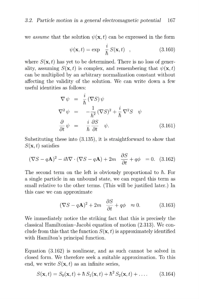
we assume that the solution ψ(x, t) can be expressed in the form
i
ψ(x, t) = exp
S(x, t) ,
(3.160)
h ¯
where S(x, t) has yet to be determined. There is no loss of generality, assuming S(x, t) is complex, and remembering that ψ(x, t)
can be multiplied by an arbitrary normalization constant without
affecting the validity of the solution. We can write down a few
useful identities as follows:
i
v ψ =
(vS) ψ
h ¯
v
2 ψ = −
1 (vS)
2 +
i v
2 S ψ
h ¯
2
h ¯
∂
i ∂S
ψ =
ψ.
(3.161)
∂t
h ¯ ∂t
Substituting these into (3.135), it is straightforward to show that
S(x, t) satisfies
(vS − qA)
2 − ih ¯v · (vS − qA) + 2m
∂S + qφ = 0. (3.162)
∂t
The second term on the left is obviously proportional to h ¯. For
a single particle in an unbound state, we can regard this term as
small relative to the other terms. (This will be justified later.) In
this case we can approximate
(vS − qA)
2 + 2m
∂S + qφ ≈ 0.
(3.163)
∂t
We immediately notice the striking fact that this is precisely the
classical Hamiltonian–Jacobi equation of motion (2.313). We conclude from this that the function S(x, t) is approximately identified
with Hamilton’s principal function.
Equation (3.162) is nonlinear, and as such cannot be solved in
closed form. We therefore seek a suitable approximation. To this
end, we write S(x, t) as an infinite series,
h
2
S(x, t) = S 0 (x, t) + ¯
h S 1 (x, t) + ¯ S 2 (x, t) + . . . .
(3.164)
�
�
�
�
�
�
�
�
�
3.2. Particle motion in a general electromagnetic potential 167
we assume that the solution ψ(x, t) can be expressed in the form
i
ψ(x, t) = exp
S(x, t) ,
(3.160)
h ¯
where S(x, t) has yet to be determined. There is no loss of generality, assuming S(x, t) is complex, and remembering that ψ(x, t)
can be multiplied by an arbitrary normalization constant without
affecting the validity of the solution. We can write down a few
useful identities as follows:
i
v ψ =
(vS) ψ
h ¯
v
2 ψ = −
1 (vS)
2 +
i v
2 S ψ
h ¯
2
h ¯
∂
i ∂S
ψ =
ψ.
(3.161)
∂t
h ¯ ∂t
Substituting these into (3.135), it is straightforward to show that
S(x, t) satisfies
(vS − qA)
2 − ih ¯v · (vS − qA) + 2m
∂S + qφ = 0. (3.162)
∂t
The second term on the left is obviously proportional to h ¯. For
a single particle in an unbound state, we can regard this term as
small relative to the other terms. (This will be justified later.) In
this case we can approximate
(vS − qA)
2 + 2m
∂S + qφ ≈ 0.
(3.163)
∂t
We immediately notice the striking fact that this is precisely the
classical Hamiltonian–Jacobi equation of motion (2.313). We conclude from this that the function S(x, t) is approximately identified
with Hamilton’s principal function.
Equation (3.162) is nonlinear, and as such cannot be solved in
closed form. We therefore seek a suitable approximation. To this
end, we write S(x, t) as an infinite series,
h
2
S(x, t) = S 0 (x, t) + ¯
h S 1 (x, t) + ¯ S 2 (x, t) + . . . .
(3.164)