

3.1. Quantum mechanical description of particle motion
131
which satisfies the time-dependent Schr¨ odinger equation (3.13).
The eigenfunction ψ j oscillates with an angular frequency ω j defined by
H j = hω ¯ j .
(3.21)
The angular frequency is constant for a given constant energy
eigenvalue H j , regardless of the form of the electrostatic potential
φ(x), assuming the potential has no explicit time dependence.
We will now proceed to derive two general mathematical properties of u j and H j , which will greatly simplify the discussion to
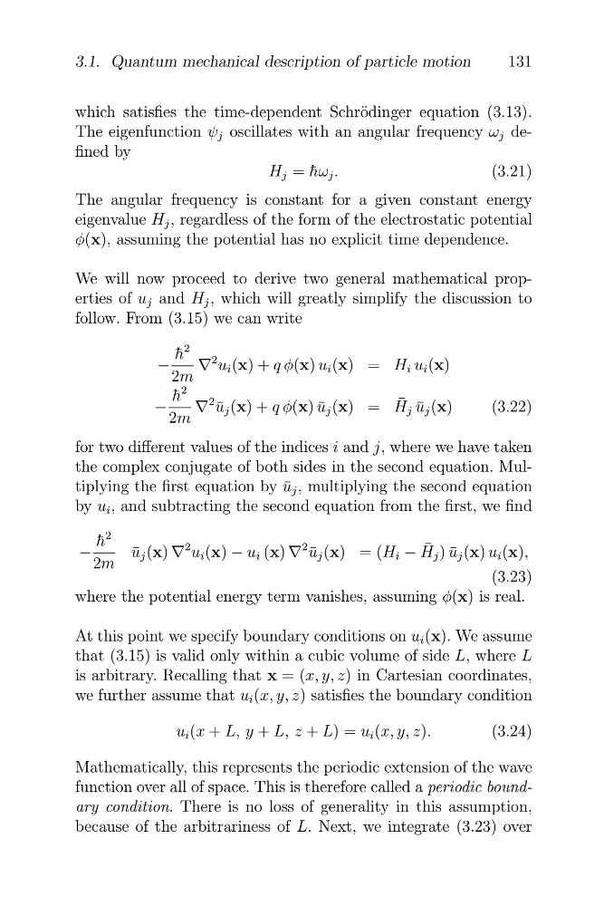
follow. From (3.15) we can write
h ¯
2
−
v
2 u i (x) + q φ(x) u i (x) = H i u i (x)
2m
h ¯
2
−
v
2
¯
u ¯ j (x) + q φ(x) u ¯ j (x) = H
m
j u ¯ j (x)
(3.22)
2
for two different values of the indices i and j, where we have taken
the complex conjugate of both sides in the second equation. Multiplying the first equation by u ¯ j , multiplying the second equation
by u i , and subtracting the second equation from the first, we find
h ¯
2
−
¯
u ¯ j (x) v
2 u i (x) − u i (x) v
2 u ¯ j (x) = (H i − H j ) u ¯ j (x) u i (x),
2m
(3.23)
where the potential energy term vanishes, assuming φ(x) is real.
At this point we specify boundary conditions on u i (x). We assume
that (3.15) is valid only within a cubic volume of side L, where L
is arbitrary. Recalling that x = (x, y, z) in Cartesian coordinates,
we further assume that u i (x, y, z) satisfies the boundary condition
u i (x + L, y + L, z + L) = u i (x, y, z).
(3.24)
Mathematically, this represents the periodic extension of the wave
function over all of space. This is therefore called a periodic boundary condition. There is no loss of generality in this assumption,
because of the arbitrariness of L. Next, we integrate (3.23) over
131
which satisfies the time-dependent Schr¨ odinger equation (3.13).
The eigenfunction ψ j oscillates with an angular frequency ω j defined by
H j = hω ¯ j .
(3.21)
The angular frequency is constant for a given constant energy
eigenvalue H j , regardless of the form of the electrostatic potential
φ(x), assuming the potential has no explicit time dependence.
We will now proceed to derive two general mathematical properties of u j and H j , which will greatly simplify the discussion to
follow. From (3.15) we can write
h ¯
2
−
v
2 u i (x) + q φ(x) u i (x) = H i u i (x)
2m
h ¯
2
−
v
2
¯
u ¯ j (x) + q φ(x) u ¯ j (x) = H
m
j u ¯ j (x)
(3.22)
2
for two different values of the indices i and j, where we have taken
the complex conjugate of both sides in the second equation. Multiplying the first equation by u ¯ j , multiplying the second equation
by u i , and subtracting the second equation from the first, we find
h ¯
2
−
¯
u ¯ j (x) v
2 u i (x) − u i (x) v
2 u ¯ j (x) = (H i − H j ) u ¯ j (x) u i (x),
2m
(3.23)
where the potential energy term vanishes, assuming φ(x) is real.
At this point we specify boundary conditions on u i (x). We assume
that (3.15) is valid only within a cubic volume of side L, where L
is arbitrary. Recalling that x = (x, y, z) in Cartesian coordinates,
we further assume that u i (x, y, z) satisfies the boundary condition
u i (x + L, y + L, z + L) = u i (x, y, z).
(3.24)
Mathematically, this represents the periodic extension of the wave
function over all of space. This is therefore called a periodic boundary condition. There is no loss of generality in this assumption,
because of the arbitrariness of L. Next, we integrate (3.23) over