

130
Chapter 3. Wave optics
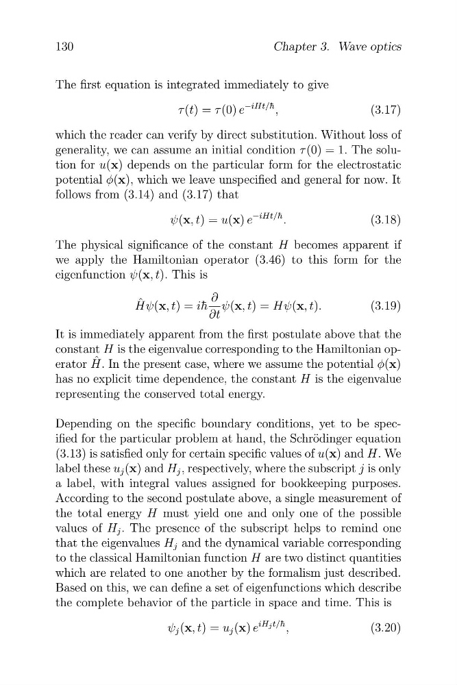
The first equation is integrated immediately to give
−iHt/¯ h
τ (t) = τ (0) e
,
(3.17)
which the reader can verify by direct substitution. Without loss of
generality, we can assume an initial condition τ (0) = 1. The solution for u(x) depends on the particular form for the electrostatic
potential φ(x), which we leave unspecified and general for now. It
follows from (3.14) and (3.17) that
−iHt/¯ h
ψ(x, t) = u(x) e
.
(3.18)
The physical significance of the constant H becomes apparent if
we apply the Hamiltonian operator (3.46) to this form for the
eigenfunction ψ(x, t). This is
∂
ˆ
Hψ(x, t) = ih ¯ ψ(x, t) = Hψ(x, t).
(3.19)
∂t
It is immediately apparent from the first postulate above that the
constant H is the eigenvalue corresponding to the Hamiltonian opˆ
erator H. In the present case, where we assume the potential φ(x)
has no explicit time dependence, the constant H is the eigenvalue
representing the conserved total energy.
Depending on the specific boundary conditions, yet to be specified for the particular problem at hand, the Schr¨ odinger equation
(3.13) is satisfied only for certain specific values of u(x) and H. We
label these u j (x) and H j , respectively, where the subscript j is only
a label, with integral values assigned for bookkeeping purposes.
According to the second postulate above, a single measurement of
the total energy H must yield one and only one of the possible
values of H j . The presence of the subscript helps to remind one
that the eigenvalues H j and the dynamical variable corresponding
to the classical Hamiltonian function H are two distinct quantities
which are related to one another by the formalism just described.
Based on this, we can define a set of eigenfunctions which describe
the complete behavior of the particle in space and time. This is
iH j t/¯ h
ψ j (x, t) = u j (x) e
,
(3.20)
Chapter 3. Wave optics
The first equation is integrated immediately to give
−iHt/¯ h
τ (t) = τ (0) e
,
(3.17)
which the reader can verify by direct substitution. Without loss of
generality, we can assume an initial condition τ (0) = 1. The solution for u(x) depends on the particular form for the electrostatic
potential φ(x), which we leave unspecified and general for now. It
follows from (3.14) and (3.17) that
−iHt/¯ h
ψ(x, t) = u(x) e
.
(3.18)
The physical significance of the constant H becomes apparent if
we apply the Hamiltonian operator (3.46) to this form for the
eigenfunction ψ(x, t). This is
∂
ˆ
Hψ(x, t) = ih ¯ ψ(x, t) = Hψ(x, t).
(3.19)
∂t
It is immediately apparent from the first postulate above that the
constant H is the eigenvalue corresponding to the Hamiltonian opˆ
erator H. In the present case, where we assume the potential φ(x)
has no explicit time dependence, the constant H is the eigenvalue
representing the conserved total energy.
Depending on the specific boundary conditions, yet to be specified for the particular problem at hand, the Schr¨ odinger equation
(3.13) is satisfied only for certain specific values of u(x) and H. We
label these u j (x) and H j , respectively, where the subscript j is only
a label, with integral values assigned for bookkeeping purposes.
According to the second postulate above, a single measurement of
the total energy H must yield one and only one of the possible
values of H j . The presence of the subscript helps to remind one
that the eigenvalues H j and the dynamical variable corresponding
to the classical Hamiltonian function H are two distinct quantities
which are related to one another by the formalism just described.
Based on this, we can define a set of eigenfunctions which describe
the complete behavior of the particle in space and time. This is
iH j t/¯ h
ψ j (x, t) = u j (x) e
,
(3.20)