

�
�
114
Chapter 2. Geometrical optics
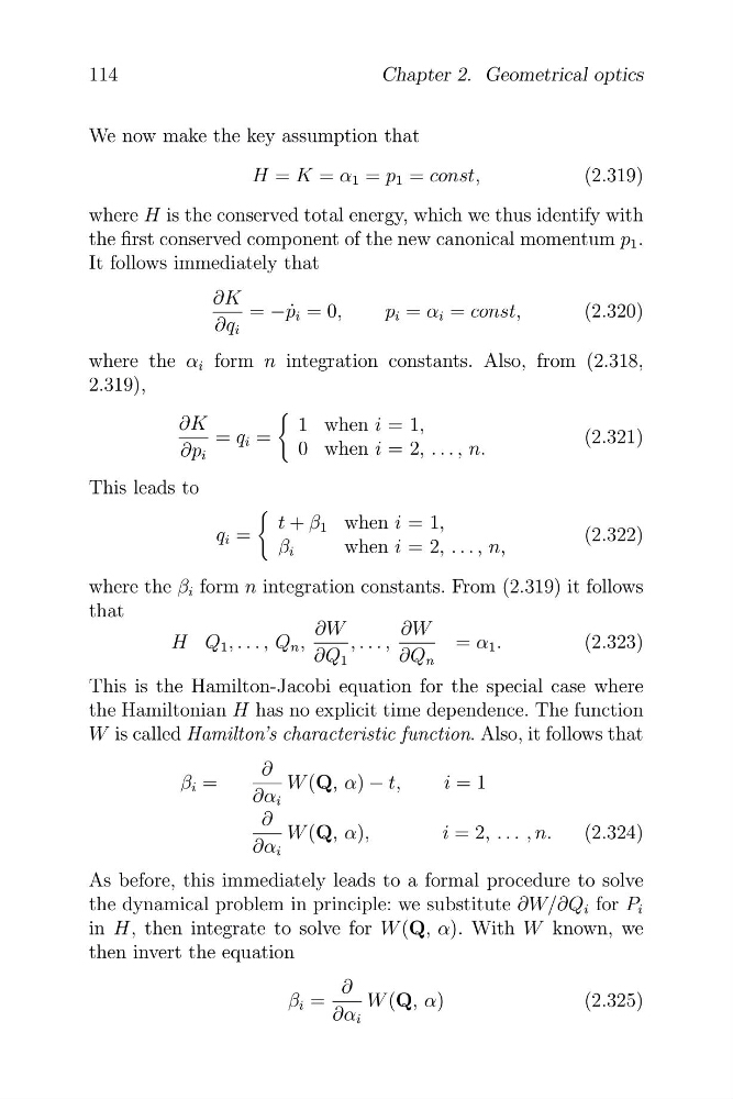
We now make the key assumption that
H = K = α 1 = p 1 = const,
(2.319)
where H is the conserved total energy, which we thus identify with
the first conserved component of the new canonical momentum p 1 .
It follows immediately that
∂K = −p ˙ i = 0,
p i = α i = const,
(2.320)
∂q i
where the α i form n integration constants. Also, from (2.318,
2.319),
∂K
1 when i = 1,
= q i =
(2.321)
∂p i
0 when i = 2, . . . , n.
This leads to
t + β 1 when i = 1,
q i =
(2.322)
β i
when i = 2, . . . , n,
where the β i form n integration constants. From (2.319) it follows
that
∂W
∂W
H Q 1 , . . . , Q n ,
, . . . ,
= α 1 .
(2.323)
∂Q 1
∂Q n
This is the Hamilton-Jacobi equation for the special case where
the Hamiltonian H has no explicit time dependence. The function
W is called Hamilton’s characteristic function. Also, it follows that
∂
β i =
W (Q, α) − t,
i = 1
∂α i
∂
W (Q, α),
i = 2, . . . , n.
(2.324)
∂α i
As before, this immediately leads to a formal procedure to solve
the dynamical problem in principle: we substitute ∂W/∂Q i for P i
in H, then integrate to solve for W (Q, α). With W known, we
then invert the equation
∂
β i =
W (Q, α)
(2.325)
∂α i
�
114
Chapter 2. Geometrical optics
We now make the key assumption that
H = K = α 1 = p 1 = const,
(2.319)
where H is the conserved total energy, which we thus identify with
the first conserved component of the new canonical momentum p 1 .
It follows immediately that
∂K = −p ˙ i = 0,
p i = α i = const,
(2.320)
∂q i
where the α i form n integration constants. Also, from (2.318,
2.319),
∂K
1 when i = 1,
= q i =
(2.321)
∂p i
0 when i = 2, . . . , n.
This leads to
t + β 1 when i = 1,
q i =
(2.322)
β i
when i = 2, . . . , n,
where the β i form n integration constants. From (2.319) it follows
that
∂W
∂W
H Q 1 , . . . , Q n ,
, . . . ,
= α 1 .
(2.323)
∂Q 1
∂Q n
This is the Hamilton-Jacobi equation for the special case where
the Hamiltonian H has no explicit time dependence. The function
W is called Hamilton’s characteristic function. Also, it follows that
∂
β i =
W (Q, α) − t,
i = 1
∂α i
∂
W (Q, α),
i = 2, . . . , n.
(2.324)
∂α i
As before, this immediately leads to a formal procedure to solve
the dynamical problem in principle: we substitute ∂W/∂Q i for P i
in H, then integrate to solve for W (Q, α). With W known, we
then invert the equation
∂
β i =
W (Q, α)
(2.325)
∂α i