

6 Synthesis of Majority Expressions Through Primitive Function Manipulation
153
Table 6.17 Example of f 1 ’s
and f 2 ’s generation by
Shannon theorem
Minterms B
C
D
E
f 1
f 2
0
0
0
0
0
0
0
1
0
0
0
1
1
0
2
0
0
1
0
1
0
3
0
0
1
1
1
0
4
0
1
0
0
0
1
5
0
1
0
1
0
1
6
0
1
1
0
0
1
7
0
1
1
1
1
0
8
1
0
0
0
1
0
9
1
0
0
1
0
1
10
1
0
1
0
0
0
11
1
0
1
1
0
1
12
1
1
0
0
1
0
13
1
1
0
1
0
1
14
1
1
1
0
1
0
15
1
1
1
1
0
1
The first step to apply this equation in the MP C algorithm is to isolate the first
input (A). Then split the input truth table f in two pieces to form 2 new truth tables,
f 1 and f 2 .
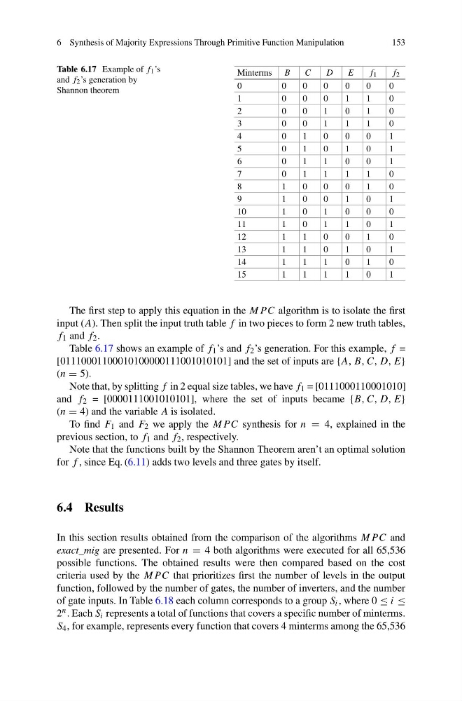
Table 6.17 shows an example of f 1 ’s and f 2 ’s generation. For this example, f =
[01110001100010100000111001010101] and the set of inputs are {A, B, C, D, E}
(n = 5).
Note that, by splitting f in 2 equal size tables, we have f 1 = [0111000110001010]
and f 2 = [0000111001010101], where the set of inputs became {B, C, D, E}
(n = 4) and the variable A is isolated.
To find F 1 and F 2 we apply the MP C synthesis for n = 4, explained in the
previous section, to f 1 and f 2 , respectively.
Note that the functions built by the Shannon Theorem aren’t an optimal solution
for f , since Eq. (6.11) adds two levels and three gates by itself.
6.4 Results
In this section results obtained from the comparison of the algorithms MP C and
exact_mig are presented. For n = 4 both algorithms were executed for all 65,536
possible functions. The obtained results were then compared based on the cost
criteria used by the MP C that prioritizes first the number of levels in the output
function, followed by the number of gates, the number of inverters, and the number
of gate inputs. In Table 6.18 each column corresponds to a group S i , where 0 ≤ i ≤
2 n . Each S i represents a total of functions that covers a specific number of minterms.
S 4 , for example, represents every function that covers 4 minterms among the 65,536
153
Table 6.17 Example of f 1 ’s
and f 2 ’s generation by
Shannon theorem
Minterms B
C
D
E
f 1
f 2
0
0
0
0
0
0
0
1
0
0
0
1
1
0
2
0
0
1
0
1
0
3
0
0
1
1
1
0
4
0
1
0
0
0
1
5
0
1
0
1
0
1
6
0
1
1
0
0
1
7
0
1
1
1
1
0
8
1
0
0
0
1
0
9
1
0
0
1
0
1
10
1
0
1
0
0
0
11
1
0
1
1
0
1
12
1
1
0
0
1
0
13
1
1
0
1
0
1
14
1
1
1
0
1
0
15
1
1
1
1
0
1
The first step to apply this equation in the MP C algorithm is to isolate the first
input (A). Then split the input truth table f in two pieces to form 2 new truth tables,
f 1 and f 2 .
Table 6.17 shows an example of f 1 ’s and f 2 ’s generation. For this example, f =
[01110001100010100000111001010101] and the set of inputs are {A, B, C, D, E}
(n = 5).
Note that, by splitting f in 2 equal size tables, we have f 1 = [0111000110001010]
and f 2 = [0000111001010101], where the set of inputs became {B, C, D, E}
(n = 4) and the variable A is isolated.
To find F 1 and F 2 we apply the MP C synthesis for n = 4, explained in the
previous section, to f 1 and f 2 , respectively.
Note that the functions built by the Shannon Theorem aren’t an optimal solution
for f , since Eq. (6.11) adds two levels and three gates by itself.
6.4 Results
In this section results obtained from the comparison of the algorithms MP C and
exact_mig are presented. For n = 4 both algorithms were executed for all 65,536
possible functions. The obtained results were then compared based on the cost
criteria used by the MP C that prioritizes first the number of levels in the output
function, followed by the number of gates, the number of inverters, and the number
of gate inputs. In Table 6.18 each column corresponds to a group S i , where 0 ≤ i ≤
2 n . Each S i represents a total of functions that covers a specific number of minterms.
S 4 , for example, represents every function that covers 4 minterms among the 65,536