

154
E. C. Ferraz et al.
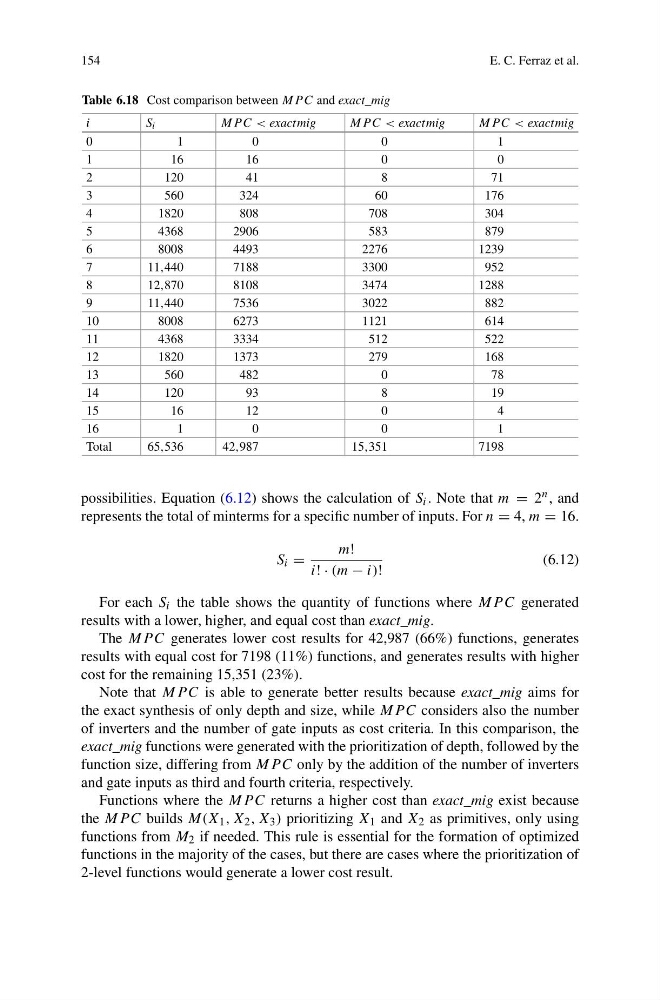
Table 6.18 Cost comparison between MP C and exact_mig
i
S i
MP C < exactmig
MP C < exactmig
MP C < exactmig
0
1
0
0
1
1
16
16
0
0
2
120
41
8
71
3
560
324
60
176
4
1820
808
708
304
5
4368
2906
583
879
6
8008
4493
2276
1239
7
11,440
7188
3300
952
8
12,870
8108
3474
1288
9
11,440
7536
3022
882
10
8008
6273
1121
614
11
4368
3334
512
522
12
1820
1373
279
168
13
560
482
0
78
14
120
93
8
19
15
16
12
0
4
16
1
0
0
1
Total
65,536
42,987
15,351
7198
possibilities. Equation (6.12) shows the calculation of S i . Note that m = 2 n , and
represents the total of minterms for a specific number of inputs. For n = 4, m = 16.
S i =
m!
i! · (m − i)!
(6.12)
For each S i the table shows the quantity of functions where MP C generated
results with a lower, higher, and equal cost than exact_mig.
The MP C generates lower cost results for 42,987 (66%) functions, generates
results with equal cost for 7198 (11%) functions, and generates results with higher
cost for the remaining 15,351 (23%).
Note that MP C is able to generate better results because exact_mig aims for
the exact synthesis of only depth and size, while MP C considers also the number
of inverters and the number of gate inputs as cost criteria. In this comparison, the
exact_mig functions were generated with the prioritization of depth, followed by the
function size, differing from MP C only by the addition of the number of inverters
and gate inputs as third and fourth criteria, respectively.
Functions where the MP C returns a higher cost than exact_mig exist because
the MP C builds M(X 1 , X 2 , X 3 ) prioritizing X 1 and X 2 as primitives, only using
functions from M 2 if needed. This rule is essential for the formation of optimized
functions in the majority of the cases, but there are cases where the prioritization of
2-level functions would generate a lower cost result.
E. C. Ferraz et al.
Table 6.18 Cost comparison between MP C and exact_mig
i
S i
MP C < exactmig
MP C < exactmig
MP C < exactmig
0
1
0
0
1
1
16
16
0
0
2
120
41
8
71
3
560
324
60
176
4
1820
808
708
304
5
4368
2906
583
879
6
8008
4493
2276
1239
7
11,440
7188
3300
952
8
12,870
8108
3474
1288
9
11,440
7536
3022
882
10
8008
6273
1121
614
11
4368
3334
512
522
12
1820
1373
279
168
13
560
482
0
78
14
120
93
8
19
15
16
12
0
4
16
1
0
0
1
Total
65,536
42,987
15,351
7198
possibilities. Equation (6.12) shows the calculation of S i . Note that m = 2 n , and
represents the total of minterms for a specific number of inputs. For n = 4, m = 16.
S i =
m!
i! · (m − i)!
(6.12)
For each S i the table shows the quantity of functions where MP C generated
results with a lower, higher, and equal cost than exact_mig.
The MP C generates lower cost results for 42,987 (66%) functions, generates
results with equal cost for 7198 (11%) functions, and generates results with higher
cost for the remaining 15,351 (23%).
Note that MP C is able to generate better results because exact_mig aims for
the exact synthesis of only depth and size, while MP C considers also the number
of inverters and the number of gate inputs as cost criteria. In this comparison, the
exact_mig functions were generated with the prioritization of depth, followed by the
function size, differing from MP C only by the addition of the number of inverters
and gate inputs as third and fourth criteria, respectively.
Functions where the MP C returns a higher cost than exact_mig exist because
the MP C builds M(X 1 , X 2 , X 3 ) prioritizing X 1 and X 2 as primitives, only using
functions from M 2 if needed. This rule is essential for the formation of optimized
functions in the majority of the cases, but there are cases where the prioritization of
2-level functions would generate a lower cost result.