

6.5 An Example: The B.C.S. Model of Superconductivity
163
where the usual notation X
J
(ξ) :=
p∈J π p (X (ξ)) was used, cf. also (6.4.12). The
generator Q ω is a well defined selfadjoint operator on the space H ω of the representation π ω chosen so that Q ω ω = 0 on the cyclic vector ω . This is the meaning
of the Bogoliubov-Haag Hamiltonian operator Q ω in the GNS-representations of
macroscopically pure and macroscopically stationary states of the system.
6.5.5 The KMS-states of (A; τ
Q
) at positive temperature T > 0:
The algebra A is separable, hence the representation space H ω of any cyclic
representation is separable and the KMS-states ω of this system are supported by
the extremal KMS states. This means, roughly speaking, that any KMS-state can be
constructed as an integral of the extremal KMS states at the same temperature T .
Hence, the evaluation of all extremal KMS states is sufficient to characterization of
all KMS states of the system. Let us consider now the extremal KMS states.
Any extremal τ
Q -KMS state at T > 0 (hence at β := T
−1
= ∞) is determined
uniquely by its restriction ω
0 to A 0 , cf. Theorem 6.4.10 (remember that all states
on the UHF-algebra A are locally normal). Let F ω ∈ g
∗ be the classical phase point
corresponding to a given extremal τ
Q -KMS state on A. Then the strong version
(6.4.29) of the ‘consistency condition’ is valid, i.e.
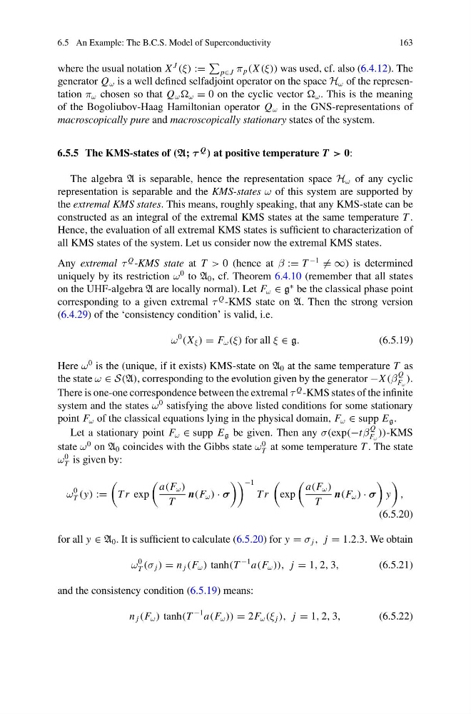
ω
0
(X ξ ) = F ω (ξ) for all ξ ∈ g.
(6.5.19)
Here ω
0 is the (unique, if it exists) KMS-state on A 0 at the same temperature T as
the state ω ∈ S(A), corresponding to the evolution given by the generator −X (β
Q
F ω
).
There is one-one correspondence between the extremal τ
Q -KMS states of the infinite
system and the states ω
0 satisfying the above listed conditions for some stationary
point F ω of the classical equations lying in the physical domain, F ω ∈ supp E g .
Let a stationary point F ω ∈ supp E g be given. Then any σ(exp(−tβ
Q
F ω
))-KMS
state ω
0 on A 0 coincides with the Gibbs state ω
0
T at some temperature T . The state
ω
0
T is given by:
ω
0
T (y) :=
T r exp
a(F ω )
T
n(F ω ) · σ
−1
T r
exp
a(F ω )
T
n(F ω ) · σ
y
,
(6.5.20)
for all y ∈ A 0 . It is sufficient to calculate (6.5.20) for y = σ j , j = 1.2.3. We obtain
ω
0
T (σ j ) = n j (F ω ) tanh(T
−1 a(F ω )), j = 1, 2, 3,
(6.5.21)
and the consistency condition (6.5.19) means:
n j (F ω ) tanh(T
−1 a(F ω )) = 2F ω (ξ j ), j = 1, 2, 3,
(6.5.22)
163
where the usual notation X
J
(ξ) :=
p∈J π p (X (ξ)) was used, cf. also (6.4.12). The
generator Q ω is a well defined selfadjoint operator on the space H ω of the representation π ω chosen so that Q ω ω = 0 on the cyclic vector ω . This is the meaning
of the Bogoliubov-Haag Hamiltonian operator Q ω in the GNS-representations of
macroscopically pure and macroscopically stationary states of the system.
6.5.5 The KMS-states of (A; τ
Q
) at positive temperature T > 0:
The algebra A is separable, hence the representation space H ω of any cyclic
representation is separable and the KMS-states ω of this system are supported by
the extremal KMS states. This means, roughly speaking, that any KMS-state can be
constructed as an integral of the extremal KMS states at the same temperature T .
Hence, the evaluation of all extremal KMS states is sufficient to characterization of
all KMS states of the system. Let us consider now the extremal KMS states.
Any extremal τ
Q -KMS state at T > 0 (hence at β := T
−1
= ∞) is determined
uniquely by its restriction ω
0 to A 0 , cf. Theorem 6.4.10 (remember that all states
on the UHF-algebra A are locally normal). Let F ω ∈ g
∗ be the classical phase point
corresponding to a given extremal τ
Q -KMS state on A. Then the strong version
(6.4.29) of the ‘consistency condition’ is valid, i.e.
ω
0
(X ξ ) = F ω (ξ) for all ξ ∈ g.
(6.5.19)
Here ω
0 is the (unique, if it exists) KMS-state on A 0 at the same temperature T as
the state ω ∈ S(A), corresponding to the evolution given by the generator −X (β
Q
F ω
).
There is one-one correspondence between the extremal τ
Q -KMS states of the infinite
system and the states ω
0 satisfying the above listed conditions for some stationary
point F ω of the classical equations lying in the physical domain, F ω ∈ supp E g .
Let a stationary point F ω ∈ supp E g be given. Then any σ(exp(−tβ
Q
F ω
))-KMS
state ω
0 on A 0 coincides with the Gibbs state ω
0
T at some temperature T . The state
ω
0
T is given by:
ω
0
T (y) :=
T r exp
a(F ω )
T
n(F ω ) · σ
−1
T r
exp
a(F ω )
T
n(F ω ) · σ
y
,
(6.5.20)
for all y ∈ A 0 . It is sufficient to calculate (6.5.20) for y = σ j , j = 1.2.3. We obtain
ω
0
T (σ j ) = n j (F ω ) tanh(T
−1 a(F ω )), j = 1, 2, 3,
(6.5.21)
and the consistency condition (6.5.19) means:
n j (F ω ) tanh(T
−1 a(F ω )) = 2F ω (ξ j ), j = 1, 2, 3,
(6.5.22)