

164
6 Dynamics of Quantum Mechanical Macroscopic Systems
which is equivalent to the following conditions:
λF ω (ξ j )
a(F ω )
tanh(T
−1 a(F ω )) = 2F ω (ξ j ), j = 1, 2;
(6.5.23a)
ε
a(F ω )
tanh(T
−1 a(F ω )) = 2F ω (ξ 3 ).
(6.5.23b)
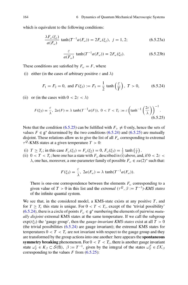
These conditions are satisfied by F ω = F, where
(i) either (in the cases of arbitrary positive ε and λ)
F 1 = F 2 = 0, and F(ξ 3 ) := F 3 =
1
2
tanh
ε
T
, T > 0,
(6.5.24)
(ii) or (in the cases with 0 < 2ε < λ)
F(ξ 3 ) =
ε
λ
, 2a(F) = λ tanh(T −1 a(F)), 0 < T < T c := ε
tanh −1
2ε
λ
−1
.
(6.5.25)
Note that the condition (6.5.25) can be fulfilled with F + = 0 only, hence the sets of
values F ∈ g
∗ determined by the two conditions (6.5.24) and (6.5.25) are mutually
disjoint. These relations allow us to give the list of all F ω corresponding to extremal
τ
Q -KMS states at a given temperature T > 0:
(i) T ≥ T c ; in this case F ω (ξ 1 ) = F ω (ξ 2 ) = 0, F ω (ξ 3 ) =
1
2
tanh
ε
T
.
(ii) 0 < T < T c ; here one has a state with F ω described in (i) above, and, if 0 < 2ε <
λ, one has, moreover, a one-parameter family of possible F ω ∈ su(2)
∗ such that:
F(ξ 3 ) =
ε
λ
, 2a(F ω ) = λ tanh(T
−1 a(F ω )).
There is one-one correspondence between the elements F ω corresponding to a
given value of T > 0 in this list and the extremal (τ
Q
, β := T
−1
)-KMS states
of the infinite quantal system.
We see that, in the considered model, a KMS-state exists at any positive T , and
for T ≥ T c this state is unique. For 0 < T < T c , except of the ‘trivial possibility’
(6.5.24), there is a circle of points F ω ∈ g
∗ numbering the elements of pairwise mutually disjoint extremal KMS states at the same temperature. If we call the subgroup
exp(tξ 3 ) the ‘gauge group’, then the gauge-invariant KMS-states exist at all T > 0
(the trivial possibilities (6.5.24) are gauge invariant); the extremal KMS states for
temperatures 0 < T < T c are not invariant with respect to the gauge group and they
are transformed by the group actions into one another: here appears the spontaneous
symmetry breaking phenomenon. For 0 < T < T c , there is another gauge invariant
state ω
s
T ∈ K β ⊂ S(A), β := T
−1
, given by the integral of the states ω
F
T ∈ EK β
corresponding to the values F from (6.5.25):
6 Dynamics of Quantum Mechanical Macroscopic Systems
which is equivalent to the following conditions:
λF ω (ξ j )
a(F ω )
tanh(T
−1 a(F ω )) = 2F ω (ξ j ), j = 1, 2;
(6.5.23a)
ε
a(F ω )
tanh(T
−1 a(F ω )) = 2F ω (ξ 3 ).
(6.5.23b)
These conditions are satisfied by F ω = F, where
(i) either (in the cases of arbitrary positive ε and λ)
F 1 = F 2 = 0, and F(ξ 3 ) := F 3 =
1
2
tanh
ε
T
, T > 0,
(6.5.24)
(ii) or (in the cases with 0 < 2ε < λ)
F(ξ 3 ) =
ε
λ
, 2a(F) = λ tanh(T −1 a(F)), 0 < T < T c := ε
tanh −1
2ε
λ
−1
.
(6.5.25)
Note that the condition (6.5.25) can be fulfilled with F + = 0 only, hence the sets of
values F ∈ g
∗ determined by the two conditions (6.5.24) and (6.5.25) are mutually
disjoint. These relations allow us to give the list of all F ω corresponding to extremal
τ
Q -KMS states at a given temperature T > 0:
(i) T ≥ T c ; in this case F ω (ξ 1 ) = F ω (ξ 2 ) = 0, F ω (ξ 3 ) =
1
2
tanh
ε
T
.
(ii) 0 < T < T c ; here one has a state with F ω described in (i) above, and, if 0 < 2ε <
λ, one has, moreover, a one-parameter family of possible F ω ∈ su(2)
∗ such that:
F(ξ 3 ) =
ε
λ
, 2a(F ω ) = λ tanh(T
−1 a(F ω )).
There is one-one correspondence between the elements F ω corresponding to a
given value of T > 0 in this list and the extremal (τ
Q
, β := T
−1
)-KMS states
of the infinite quantal system.
We see that, in the considered model, a KMS-state exists at any positive T , and
for T ≥ T c this state is unique. For 0 < T < T c , except of the ‘trivial possibility’
(6.5.24), there is a circle of points F ω ∈ g
∗ numbering the elements of pairwise mutually disjoint extremal KMS states at the same temperature. If we call the subgroup
exp(tξ 3 ) the ‘gauge group’, then the gauge-invariant KMS-states exist at all T > 0
(the trivial possibilities (6.5.24) are gauge invariant); the extremal KMS states for
temperatures 0 < T < T c are not invariant with respect to the gauge group and they
are transformed by the group actions into one another: here appears the spontaneous
symmetry breaking phenomenon. For 0 < T < T c , there is another gauge invariant
state ω
s
T ∈ K β ⊂ S(A), β := T
−1
, given by the integral of the states ω
F
T ∈ EK β
corresponding to the values F from (6.5.25):