

94
5 Finite Element Formulations
1 K uu =
B
T
u H c B u d,
(5.86)
1 K uφ =
B
T
u H
T
e B φ + 2B
T
u H
T
b
1
0 | ¯
E|B φ
d,
(5.87)
1 F ui =
B
T
u H c
1
0 S + B
T
u H
T
e
1
0 E + B
T
u H
T
b
1
0 | ¯
E|
1
0 E
d,
(5.88)
1 K φu =
B
T
φ H e B u d,
(5.89)
1 K φφ =
B
T
φ H g B φ + 2B
T
φ H h
1
0 | ¯
E|B φ
d,
(5.90)
1 G φi =
B
T
φ H e
1
0 S + B
T
φ H g
1
0 E + B
T
φ H h
1
0 | ¯
E|
1
0 E
d.
(5.91)
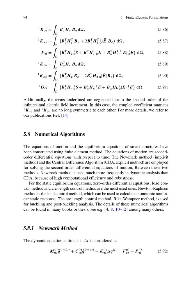
Additionally, the terms underlined are neglected due to the second order of the
infinitesimal electric field increment. In this case, the coupled coefficient matrices
1 K uφ and
1 K φu are no long symmetric to each other. For more details, we refer to
our publications Ref. [14].
5.8 Numerical Algorithms
The equations of motion and the equilibrium equations of smart structures have
been constructed using finite element method. The equations of motion are secondorder differential equations with respect to time. The Newmark method (implicit
method) and the Central Difference Algorithm (CDA, explicit method) are employed
for solving the second-order differential equations of motion. Between these two
methods, Newmark method is used much more frequently in dynamic analysis than
CDA, because of high computational efficiency and robustness.
For the static equilibrium equations, zero-order differential equations, load control method and arc-length control method are the most used ones. Newton-Raphson
method is the load control method, which can be used to calculate monotonic nonlinear static response. The arc-length control method, Riks-Wempner method, is used
for buckling and post-buckling analysis. The details of these numerical algorithms
can be found in many books or thesis, see e.g. [4, 8, 10–12] among many others.
5.8.1 Newmark Method
The dynamic equation at time t + Δt is considered as
M
(t)
uu ¨
q
(t+Δt) + C
(t)
uu ˙
q
(t+Δt) + K
(t)
uu q
(t)
= F
(t)
ue − F
(t)
ui
(5.92)
5 Finite Element Formulations
1 K uu =
B
T
u H c B u d,
(5.86)
1 K uφ =
B
T
u H
T
e B φ + 2B
T
u H
T
b
1
0 | ¯
E|B φ
d,
(5.87)
1 F ui =
B
T
u H c
1
0 S + B
T
u H
T
e
1
0 E + B
T
u H
T
b
1
0 | ¯
E|
1
0 E
d,
(5.88)
1 K φu =
B
T
φ H e B u d,
(5.89)
1 K φφ =
B
T
φ H g B φ + 2B
T
φ H h
1
0 | ¯
E|B φ
d,
(5.90)
1 G φi =
B
T
φ H e
1
0 S + B
T
φ H g
1
0 E + B
T
φ H h
1
0 | ¯
E|
1
0 E
d.
(5.91)
Additionally, the terms underlined are neglected due to the second order of the
infinitesimal electric field increment. In this case, the coupled coefficient matrices
1 K uφ and
1 K φu are no long symmetric to each other. For more details, we refer to
our publications Ref. [14].
5.8 Numerical Algorithms
The equations of motion and the equilibrium equations of smart structures have
been constructed using finite element method. The equations of motion are secondorder differential equations with respect to time. The Newmark method (implicit
method) and the Central Difference Algorithm (CDA, explicit method) are employed
for solving the second-order differential equations of motion. Between these two
methods, Newmark method is used much more frequently in dynamic analysis than
CDA, because of high computational efficiency and robustness.
For the static equilibrium equations, zero-order differential equations, load control method and arc-length control method are the most used ones. Newton-Raphson
method is the load control method, which can be used to calculate monotonic nonlinear static response. The arc-length control method, Riks-Wempner method, is used
for buckling and post-buckling analysis. The details of these numerical algorithms
can be found in many books or thesis, see e.g. [4, 8, 10–12] among many others.
5.8.1 Newmark Method
The dynamic equation at time t + Δt is considered as
M
(t)
uu ¨
q
(t+Δt) + C
(t)
uu ˙
q
(t+Δt) + K
(t)
uu q
(t)
= F
(t)
ue − F
(t)
ui
(5.92)