

5.7 Geometrically and Electroelastic Nonlinear FE Model
93
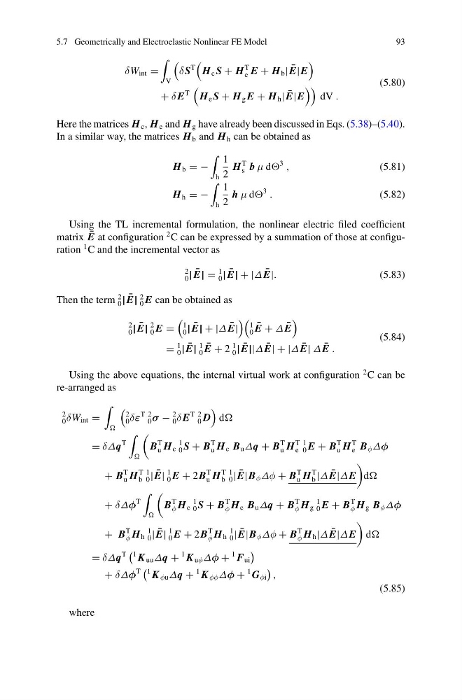
δW int =
V
δ S
T
H c S + H
T
e E + H b | ¯
E|E
+ δ E
T
H e S + H g E + H h | ¯
E|E
dV .
(5.80)
Here the matrices H c , H e and H g have already been discussed in Eqs. (5.38)–(5.40).
In a similar way, the matrices H b and H h can be obtained as
H b = −
h
1
2
H
T
s b μ d
3
,
(5.81)
H h = −
h
1
2
h μ d
3
.
(5.82)
Using the TL incremental formulation, the nonlinear electric filed coefficient
matrix ¯
E at configuration
2 C can be expressed by a summation of those at configuration
1 C and the incremental vector as
2
0 | ¯
E| =
1
0 | ¯
E| + |Δ ¯
E|.
(5.83)
Then the term
2
0 | ¯
E|
2
0 E can be obtained as
2
0 | ¯
E|
2
0 E =
1
0 | ¯
E| + |Δ ¯
E|
1
0
¯
E + Δ ¯
E
=
1
0 | ¯
E|
1
0
¯
E + 2
1
0 | ¯
E||Δ ¯
E| + |Δ ¯
E| Δ ¯
E .
(5.84)
Using the above equations, the internal virtual work at configuration
2 C can be
re-arranged as
2
0 δW int =
2
0 δε
T 2
0 σ −
2
0 δ E
T 2
0 D
d
= δΔq
T
B
T
u H c
1
0 S + B
T
u H c B u Δq + B
T
u H
T
e
1
0 E + B
T
u H
T
e B φ Δφ
+ B
T
u H
T
b
1
0 | ¯
E|
1
0 E + 2B
T
u H
T
b
1
0 | ¯
E|B φ Δφ + B
T
u H
T
b |Δ ¯
E|ΔE
d
+ δΔφ
T
B
T
φ H e
1
0 S + B
T
φ H e B u Δq + B
T
φ H g
1
0 E + B
T
φ H g B φ Δφ
+ B
T
φ H h
1
0 | ¯
E|
1
0 E + 2B
T
φ H h
1
0 | ¯
E|B φ Δφ + B
T
φ H h |Δ ¯
E|ΔE
d
= δΔq
T
1 K uu Δq +
1 K uφ Δφ +
1 F ui
+ δΔφ
T
1 K φu Δq +
1 K φφ Δφ +
1 G φi
,
(5.85)
where
93
δW int =
V
δ S
T
H c S + H
T
e E + H b | ¯
E|E
+ δ E
T
H e S + H g E + H h | ¯
E|E
dV .
(5.80)
Here the matrices H c , H e and H g have already been discussed in Eqs. (5.38)–(5.40).
In a similar way, the matrices H b and H h can be obtained as
H b = −
h
1
2
H
T
s b μ d
3
,
(5.81)
H h = −
h
1
2
h μ d
3
.
(5.82)
Using the TL incremental formulation, the nonlinear electric filed coefficient
matrix ¯
E at configuration
2 C can be expressed by a summation of those at configuration
1 C and the incremental vector as
2
0 | ¯
E| =
1
0 | ¯
E| + |Δ ¯
E|.
(5.83)
Then the term
2
0 | ¯
E|
2
0 E can be obtained as
2
0 | ¯
E|
2
0 E =
1
0 | ¯
E| + |Δ ¯
E|
1
0
¯
E + Δ ¯
E
=
1
0 | ¯
E|
1
0
¯
E + 2
1
0 | ¯
E||Δ ¯
E| + |Δ ¯
E| Δ ¯
E .
(5.84)
Using the above equations, the internal virtual work at configuration
2 C can be
re-arranged as
2
0 δW int =
2
0 δε
T 2
0 σ −
2
0 δ E
T 2
0 D
d
= δΔq
T
B
T
u H c
1
0 S + B
T
u H c B u Δq + B
T
u H
T
e
1
0 E + B
T
u H
T
e B φ Δφ
+ B
T
u H
T
b
1
0 | ¯
E|
1
0 E + 2B
T
u H
T
b
1
0 | ¯
E|B φ Δφ + B
T
u H
T
b |Δ ¯
E|ΔE
d
+ δΔφ
T
B
T
φ H e
1
0 S + B
T
φ H e B u Δq + B
T
φ H g
1
0 E + B
T
φ H g B φ Δφ
+ B
T
φ H h
1
0 | ¯
E|
1
0 E + 2B
T
φ H h
1
0 | ¯
E|B φ Δφ + B
T
φ H h |Δ ¯
E|ΔE
d
= δΔq
T
1 K uu Δq +
1 K uφ Δφ +
1 F ui
+ δΔφ
T
1 K φu Δq +
1 K φφ Δφ +
1 G φi
,
(5.85)
where