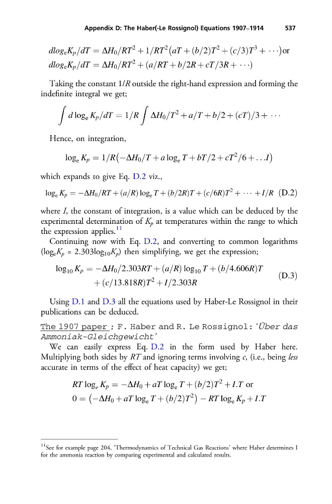
dlog e K p =dT ¼ DH 0 =RT
2
þ 1=RT
2
aT þ ðb=2ÞT
2
þ ðc=3ÞT
3
þ Á Á Á
À
Á
or
dlog e K p =dT ¼ DH 0 =RT
2
þ ða=RT þ b=2R þ cT=3R þ Á Á ÁÞ
Taking the constant 1/R outside the right-hand expression and forming the
indefinite integral we get;
Z
d log e K p =dT ¼ 1=R
Z
DH 0 =T
2
þ a=T þ b=2 þ ðcTÞ=3 þ Á Á Á
Hence, on integration,
log e K p ¼ 1=R ÀDH 0 =T þ a log e T þ bT=2 þ cT
2
=6 þ . . .I
À
Á
which expands to give Eq. D.2 viz.,
log e K p ¼ ÀDH 0 =RT þ ða=RÞ log e T þ ðb=2RÞT þ ðc=6RÞT
2
þ Á Á Á þ I=R ðD:2Þ
where I, the constant of integration, is a value which can be deduced by the
experimental determination of K p at temperatures within the range to which
the expression applies.
11
Continuing now with Eq. D.2, and converting to common logarithms
(log e K p = 2.303log 10 K p ) then simplifying, we get the expression;
log 10 K p ¼ ÀDH 0 =2:303RT þ ða=RÞ log 10 T þ ðb=4:606RÞT
þ ðc=13:818RÞT
2
þ I=2:303R
ðD:3Þ
Using D.1 and D.3 all the equations used by Haber-Le Rossignol in their
publications can be deduced.
The 1907 paper ; F. Haber and R. Le Rossignol: ‘Über das
Ammoniak-Gleichgewicht’
We can easily express Eq. D.2 in the form used by Haber here.
Multiplying both sides by RT and ignoring terms involving c, (i.e., being less
accurate in terms of the effect of heat capacity) we get;
RT log e K p ¼ ÀDH 0 þ aT log e T þ ðb=2ÞT
2
þ I:T or
0 ¼ ÀDH 0 þ aT log e T þ ðb=2ÞT
2
À
Á À RT log e K p þ I:T
11 See for example page 204, ‘Thermodynamics of Technical Gas Reactions’ where Haber determines I
for the ammonia reaction by comparing experimental and calculated results.
Appendix D: The Haber(-Le Rossignol) Equations 1907–1914
537