

log 10 K p ¼ ÀQ pðTÞ =4:571T þ
X
v 1:75 log 10 T þ
X
v I
and now with
P
v = −1, I = 1.3 and Q p(T) = −12,000 cal mole
−1 , he arrived
at;
log 10 K p ¼ 12;000=4:571 T À 1:75 log 10 T À 1:3
However, Haber decided to take into account the average specific heats of
the ammonia and ‘permanent’ gases from absolute zero to the temperatures of
the experiments, a point which Nernst had failed to address.
10 By adding the
term 0.000651T to the right hand side, the average specific heat of ammonia
at constant pressure became 9.5 + 0.004157T whilst at the same time the
increase in the average specific heat of the ‘permanent gases’ became
0.0006T. With the Nernst approximation now in the form;
log 10 K p ¼ 12;000=4:571T À 1:75 log 10 T þ 0:000651 T À 1:3
Haber presented the ‘calculated’ equilibrium constants K
Nernst eqn
p
to
which we have again added the corresponding %ammonia at equilibrium,
Table 5.4.
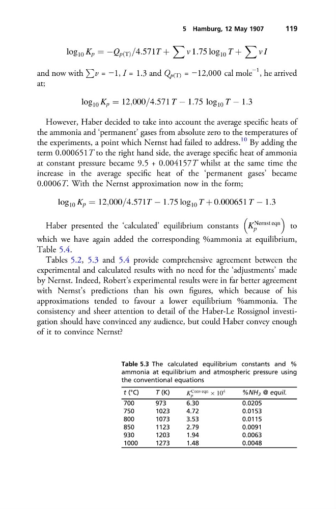
Tables 5.2, 5.3 and 5.4 provide comprehensive agreement between the
experimental and calculated results with no need for the ‘adjustments’ made
by Nernst. Indeed, Robert’s experimental results were in far better agreement
with Nernst’s predictions than his own figures, which because of his
approximations tended to favour a lower equilibrium %ammonia. The
consistency and sheer attention to detail of the Haber-Le Rossignol investigation should have convinced any audience, but could Haber convey enough
of it to convince Nernst?
Table 5.3 The calculated equilibrium constants and %
ammonia at equilibrium and atmospheric pressure using
the conventional equations
t (°C)
T (K)
K
Conv eqn
p
 10
4
%NH 3 @ equil.
700
973
6.30
0.0205
750
1023
4.72
0.0153
800
1073
3.53
0.0115
850
1123
2.79
0.0091
930
1203
1.94
0.0063
1000
1273
1.48
0.0048
5 Hamburg, 12 May 1907
119
X
v 1:75 log 10 T þ
X
v I
and now with
P
v = −1, I = 1.3 and Q p(T) = −12,000 cal mole
−1 , he arrived
at;
log 10 K p ¼ 12;000=4:571 T À 1:75 log 10 T À 1:3
However, Haber decided to take into account the average specific heats of
the ammonia and ‘permanent’ gases from absolute zero to the temperatures of
the experiments, a point which Nernst had failed to address.
10 By adding the
term 0.000651T to the right hand side, the average specific heat of ammonia
at constant pressure became 9.5 + 0.004157T whilst at the same time the
increase in the average specific heat of the ‘permanent gases’ became
0.0006T. With the Nernst approximation now in the form;
log 10 K p ¼ 12;000=4:571T À 1:75 log 10 T þ 0:000651 T À 1:3
Haber presented the ‘calculated’ equilibrium constants K
Nernst eqn
p
to
which we have again added the corresponding %ammonia at equilibrium,
Table 5.4.
Tables 5.2, 5.3 and 5.4 provide comprehensive agreement between the
experimental and calculated results with no need for the ‘adjustments’ made
by Nernst. Indeed, Robert’s experimental results were in far better agreement
with Nernst’s predictions than his own figures, which because of his
approximations tended to favour a lower equilibrium %ammonia. The
consistency and sheer attention to detail of the Haber-Le Rossignol investigation should have convinced any audience, but could Haber convey enough
of it to convince Nernst?
Table 5.3 The calculated equilibrium constants and %
ammonia at equilibrium and atmospheric pressure using
the conventional equations
t (°C)
T (K)
K
Conv eqn
p
 10
4
%NH 3 @ equil.
700
973
6.30
0.0205
750
1023
4.72
0.0153
800
1073
3.53
0.0115
850
1123
2.79
0.0091
930
1203
1.94
0.0063
1000
1273
1.48
0.0048
5 Hamburg, 12 May 1907
119