

248
6 Hierarchical Component Models
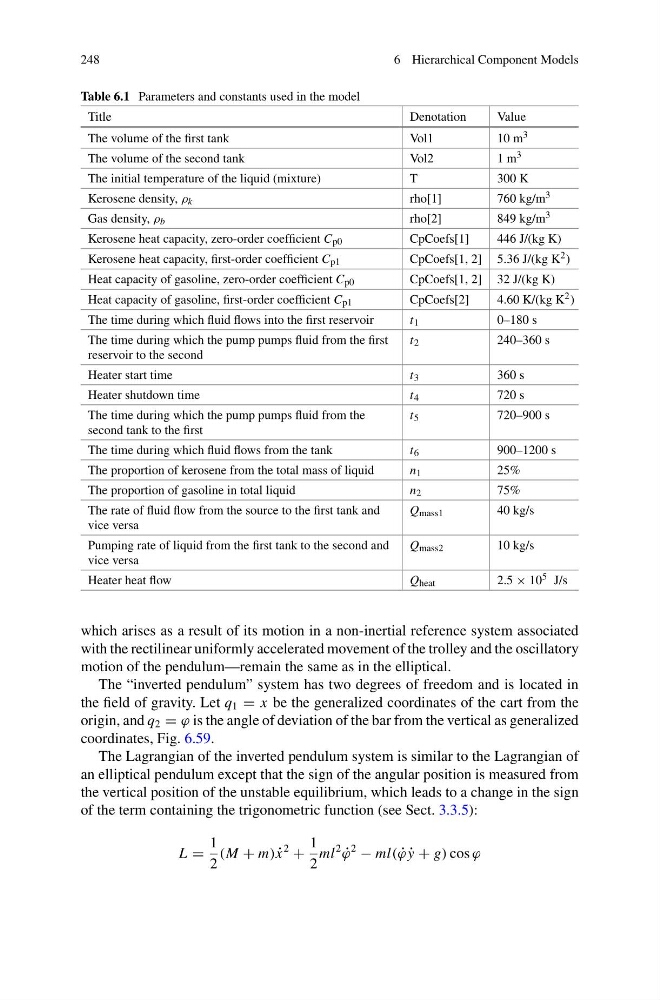
Table 6.1 Parameters and constants used in the model
Title
Denotation
Value
The volume of the first tank
Vol1
10 m 3
The volume of the second tank
Vol2
1 m 3
The initial temperature of the liquid (mixture)
T
300 K
Kerosene density, ρ k
rho[1]
760 kg/m 3
Gas density, ρ b
rho[2]
849 kg/m 3
Kerosene heat capacity, zero-order coefficient C p0
CpCoefs[1]
446 J/(kg K)
Kerosene heat capacity, first-order coefficient C p1
CpCoefs[1, 2] 5.36 J/(kg K 2 )
Heat capacity of gasoline, zero-order coefficient C p0
CpCoefs[1, 2] 32 J/(kg K)
Heat capacity of gasoline, first-order coefficient C p1
CpCoefs[2]
4.60 K/(kg K 2 )
The time during which fluid flows into the first reservoir
t 1
0–180 s
The time during which the pump pumps fluid from the first
reservoir to the second
t 2
240–360 s
Heater start time
t 3
360 s
Heater shutdown time
t 4
720 s
The time during which the pump pumps fluid from the
second tank to the first
t 5
720–900 s
The time during which fluid flows from the tank
t 6
900–1200 s
The proportion of kerosene from the total mass of liquid
n 1
25%
The proportion of gasoline in total liquid
n 2
75%
The rate of fluid flow from the source to the first tank and
vice versa
Q mass1
40 kg/s
Pumping rate of liquid from the first tank to the second and
vice versa
Q mass2
10 kg/s
Heater heat flow
Q heat
2.5 × 10 5 J/s
which arises as a result of its motion in a non-inertial reference system associated
with the rectilinear uniformly accelerated movement of the trolley and the oscillatory
motion of the pendulum—remain the same as in the elliptical.
The “inverted pendulum” system has two degrees of freedom and is located in
the field of gravity. Let q 1 = x be the generalized coordinates of the cart from the
origin, and q 2 = ϕ is the angle of deviation of the bar from the vertical as generalized
coordinates, Fig. 6.59.
The Lagrangian of the inverted pendulum system is similar to the Lagrangian of
an elliptical pendulum except that the sign of the angular position is measured from
the vertical position of the unstable equilibrium, which leads to a change in the sign
of the term containing the trigonometric function (see Sect. 3.3.5):
L =
1
2
(M + m) ˙
x
2
+
1
2
ml
2
˙
ϕ
2
− ml( ˙
ϕ ˙
y + g) cos ϕ
6 Hierarchical Component Models
Table 6.1 Parameters and constants used in the model
Title
Denotation
Value
The volume of the first tank
Vol1
10 m 3
The volume of the second tank
Vol2
1 m 3
The initial temperature of the liquid (mixture)
T
300 K
Kerosene density, ρ k
rho[1]
760 kg/m 3
Gas density, ρ b
rho[2]
849 kg/m 3
Kerosene heat capacity, zero-order coefficient C p0
CpCoefs[1]
446 J/(kg K)
Kerosene heat capacity, first-order coefficient C p1
CpCoefs[1, 2] 5.36 J/(kg K 2 )
Heat capacity of gasoline, zero-order coefficient C p0
CpCoefs[1, 2] 32 J/(kg K)
Heat capacity of gasoline, first-order coefficient C p1
CpCoefs[2]
4.60 K/(kg K 2 )
The time during which fluid flows into the first reservoir
t 1
0–180 s
The time during which the pump pumps fluid from the first
reservoir to the second
t 2
240–360 s
Heater start time
t 3
360 s
Heater shutdown time
t 4
720 s
The time during which the pump pumps fluid from the
second tank to the first
t 5
720–900 s
The time during which fluid flows from the tank
t 6
900–1200 s
The proportion of kerosene from the total mass of liquid
n 1
25%
The proportion of gasoline in total liquid
n 2
75%
The rate of fluid flow from the source to the first tank and
vice versa
Q mass1
40 kg/s
Pumping rate of liquid from the first tank to the second and
vice versa
Q mass2
10 kg/s
Heater heat flow
Q heat
2.5 × 10 5 J/s
which arises as a result of its motion in a non-inertial reference system associated
with the rectilinear uniformly accelerated movement of the trolley and the oscillatory
motion of the pendulum—remain the same as in the elliptical.
The “inverted pendulum” system has two degrees of freedom and is located in
the field of gravity. Let q 1 = x be the generalized coordinates of the cart from the
origin, and q 2 = ϕ is the angle of deviation of the bar from the vertical as generalized
coordinates, Fig. 6.59.
The Lagrangian of the inverted pendulum system is similar to the Lagrangian of
an elliptical pendulum except that the sign of the angular position is measured from
the vertical position of the unstable equilibrium, which leads to a change in the sign
of the term containing the trigonometric function (see Sect. 3.3.5):
L =
1
2
(M + m) ˙
x
2
+
1
2
ml
2
˙
ϕ
2
− ml( ˙
ϕ ˙
y + g) cos ϕ