

104
3 Computer Simulation of Dynamic Systems
m
d
2 r
dt 2 = −kr + F(r, t)
In the simplest case, the applied force F(r, t) = F 0 is constant.
We carry out the change of variables: r = r − F 0 /k. We obtain for the new
variable r :
d
2 r
dt 2 = −kr ,
i.e., a constant force does not make changes in the oscillation process, with the
exception that the coordinate of the neutral point at which the force acting on the
load is zero is shifted by the value F 0 /k. Thus, for example, a model of a vertical
spring pendulum is constructed.
A much more complex picture of motion can arise when a time-dependent force
F(t) acts on the system. For definiteness, we consider the periodic external force
F(t) = F 0 sin ω 1 t:
m
d
2 r
dt 2 = −kr + F(t) = −kr + F 0 sin ω 1 t
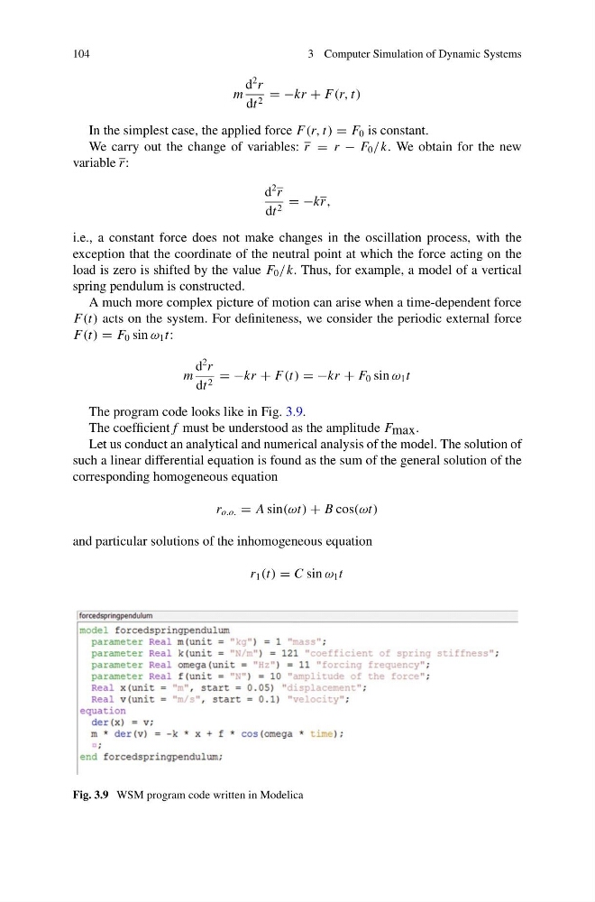
The program code looks like in Fig. 3.9.
The coefficient f must be understood as the amplitude F max .
Let us conduct an analytical and numerical analysis of the model. The solution of
such a linear differential equation is found as the sum of the general solution of the
corresponding homogeneous equation
r o.o. = A sin(ωt) + B cos(ωt)
and particular solutions of the inhomogeneous equation
r 1 (t) = C sin ω 1 t
Fig. 3.9 WSM program code written in Modelica
3 Computer Simulation of Dynamic Systems
m
d
2 r
dt 2 = −kr + F(r, t)
In the simplest case, the applied force F(r, t) = F 0 is constant.
We carry out the change of variables: r = r − F 0 /k. We obtain for the new
variable r :
d
2 r
dt 2 = −kr ,
i.e., a constant force does not make changes in the oscillation process, with the
exception that the coordinate of the neutral point at which the force acting on the
load is zero is shifted by the value F 0 /k. Thus, for example, a model of a vertical
spring pendulum is constructed.
A much more complex picture of motion can arise when a time-dependent force
F(t) acts on the system. For definiteness, we consider the periodic external force
F(t) = F 0 sin ω 1 t:
m
d
2 r
dt 2 = −kr + F(t) = −kr + F 0 sin ω 1 t
The program code looks like in Fig. 3.9.
The coefficient f must be understood as the amplitude F max .
Let us conduct an analytical and numerical analysis of the model. The solution of
such a linear differential equation is found as the sum of the general solution of the
corresponding homogeneous equation
r o.o. = A sin(ωt) + B cos(ωt)
and particular solutions of the inhomogeneous equation
r 1 (t) = C sin ω 1 t
Fig. 3.9 WSM program code written in Modelica