

98
3 Computer Simulation of Dynamic Systems
d
dε
S[r + εϕ]
ε=0
= −
t 2
t 1
ϕ
m
d
2 r
dt 2 + kr
dt = 0
Since the test function ϕ(t) is arbitrary, the part of the expression under the integral
sign in square brackets must be equal to zero at all time t 1 < t < t 2 :
m
d
2 r
dt 2 + kr = 0
such that the motion of the system must be described by the same equation that we
obtained in the previous paragraph from Newton’s law and the law of conservation
of energy. All three approaches are equivalent.
Consider another example of the application of the Hamilton principle.
Consider a mathematical pendulum—that is, a harmonic oscillator—which is a
mechanical system consisting of a material point at the end of a weightless inextensible thread or a weightless inextensible rod and located in a uniform field of gravity.
The pendulum moves in a medium without resistance.
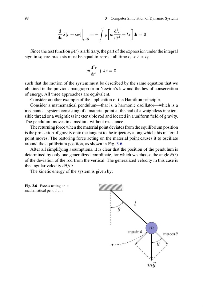
The returning force when the material point deviates from the equilibrium position
is the projection of gravity onto the tangent to the trajectory along which this material
point moves. The restoring force acting on the material point causes it to oscillate
around the equilibrium position, as shown in Fig. 3.6.
After all simplifying assumptions, it is clear that the position of the pendulum is
determined by only one generalized coordinate, for which we choose the angle θ(t)
of the deviation of the rod from the vertical. The generalized velocity in this case is
the angular velocity dθ/dt.
The kinetic energy of the system is given by:
Fig. 3.6 Forces acting on a
mathematical pendulum
3 Computer Simulation of Dynamic Systems
d
dε
S[r + εϕ]
ε=0
= −
t 2
t 1
ϕ
m
d
2 r
dt 2 + kr
dt = 0
Since the test function ϕ(t) is arbitrary, the part of the expression under the integral
sign in square brackets must be equal to zero at all time t 1 < t < t 2 :
m
d
2 r
dt 2 + kr = 0
such that the motion of the system must be described by the same equation that we
obtained in the previous paragraph from Newton’s law and the law of conservation
of energy. All three approaches are equivalent.
Consider another example of the application of the Hamilton principle.
Consider a mathematical pendulum—that is, a harmonic oscillator—which is a
mechanical system consisting of a material point at the end of a weightless inextensible thread or a weightless inextensible rod and located in a uniform field of gravity.
The pendulum moves in a medium without resistance.
The returning force when the material point deviates from the equilibrium position
is the projection of gravity onto the tangent to the trajectory along which this material
point moves. The restoring force acting on the material point causes it to oscillate
around the equilibrium position, as shown in Fig. 3.6.
After all simplifying assumptions, it is clear that the position of the pendulum is
determined by only one generalized coordinate, for which we choose the angle θ(t)
of the deviation of the rod from the vertical. The generalized velocity in this case is
the angular velocity dθ/dt.
The kinetic energy of the system is given by:
Fig. 3.6 Forces acting on a
mathematical pendulum