

3.2 Fundamental Principles for Mathematical Models Development
97
The function ϕ(t) that appears in the principle of least action is a certain test
function that vanishes at time instants t 1 , t 2 and satisfies the condition that Q(t) +
εϕ(t) is the possible coordinate of this system (otherwise, ϕ(t) arbitrary).
The meaning of the principle of least action is that of all a priori admissible
trajectories (movements) of the system between the moments t 1 , t 2 , a motion is
selected (implemented) that delivers a minimum to the action functional (the name
of the principle also comes from this). The function εϕ(t) is called a variation of the
quantity Q(t).
So, the application scheme of the Hamilton principle for constructing models
of mechanical systems is as follows: Generalized coordinates Q(t) and generalized
velocities dQ/dt of the system are determined, the Lagrange function L(Q, dQ/dt)
and the action functional S[Q] are constructed, minimization which, on the variations
εϕ(t) of the coordinate Q(t), gives the desired model.
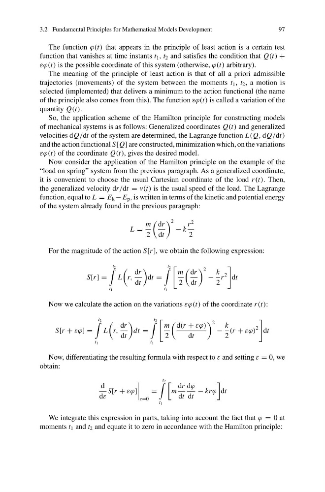
Now consider the application of the Hamilton principle on the example of the
“load on spring” system from the previous paragraph. As a generalized coordinate,
it is convenient to choose the usual Cartesian coordinate of the load r (t). Then,
the generalized velocity dr/dt = v(t) is the usual speed of the load. The Lagrange
function, equal to L = E k − E p , is written in terms of the kinetic and potential energy
of the system already found in the previous paragraph:
L =
m
2
dr
dt
2
− k
r
2
2
For the magnitude of the action S[r ], we obtain the following expression:
S[r ] =
t 2
t 1
L
r,
dr
dt
dt =
t 2
t 1
m
2
dr
dt
2
−
k
2
r
2
dt
Now we calculate the action on the variations εϕ(t) of the coordinate r (t):
S[r + εϕ] =
t 2
t 1
L
r,
dr
dt
dt =
t 2
t 1
m
2
d(r + εϕ)
dt
2
−
k
2
(r + εϕ)
2
dt
Now, differentiating the resulting formula with respect to ε and setting ε = 0, we
obtain:
d
dε
S[r + εϕ]
ε=0
=
t 2
t 1
m
dr
dt
dϕ
dt
− krϕ
dt
We integrate this expression in parts, taking into account the fact that ϕ = 0 at
moments t 1 and t 2 and equate it to zero in accordance with the Hamilton principle:
97
The function ϕ(t) that appears in the principle of least action is a certain test
function that vanishes at time instants t 1 , t 2 and satisfies the condition that Q(t) +
εϕ(t) is the possible coordinate of this system (otherwise, ϕ(t) arbitrary).
The meaning of the principle of least action is that of all a priori admissible
trajectories (movements) of the system between the moments t 1 , t 2 , a motion is
selected (implemented) that delivers a minimum to the action functional (the name
of the principle also comes from this). The function εϕ(t) is called a variation of the
quantity Q(t).
So, the application scheme of the Hamilton principle for constructing models
of mechanical systems is as follows: Generalized coordinates Q(t) and generalized
velocities dQ/dt of the system are determined, the Lagrange function L(Q, dQ/dt)
and the action functional S[Q] are constructed, minimization which, on the variations
εϕ(t) of the coordinate Q(t), gives the desired model.
Now consider the application of the Hamilton principle on the example of the
“load on spring” system from the previous paragraph. As a generalized coordinate,
it is convenient to choose the usual Cartesian coordinate of the load r (t). Then,
the generalized velocity dr/dt = v(t) is the usual speed of the load. The Lagrange
function, equal to L = E k − E p , is written in terms of the kinetic and potential energy
of the system already found in the previous paragraph:
L =
m
2
dr
dt
2
− k
r
2
2
For the magnitude of the action S[r ], we obtain the following expression:
S[r ] =
t 2
t 1
L
r,
dr
dt
dt =
t 2
t 1
m
2
dr
dt
2
−
k
2
r
2
dt
Now we calculate the action on the variations εϕ(t) of the coordinate r (t):
S[r + εϕ] =
t 2
t 1
L
r,
dr
dt
dt =
t 2
t 1
m
2
d(r + εϕ)
dt
2
−
k
2
(r + εϕ)
2
dt
Now, differentiating the resulting formula with respect to ε and setting ε = 0, we
obtain:
d
dε
S[r + εϕ]
ε=0
=
t 2
t 1
m
dr
dt
dϕ
dt
− krϕ
dt
We integrate this expression in parts, taking into account the fact that ϕ = 0 at
moments t 1 and t 2 and equate it to zero in accordance with the Hamilton principle: