

IoT in Provenance Management of Medical Data
359
Hill’s equation can fit either the descending or ascending dependences. It depends
on the sign of the Hill’s slope (d <> 0). One has expected the descending trend, so
and the negative slope [30, 33].
There are different ways of computing of Hill’s parameters [33, 34]. Here is in
use of the method [33] and the opportunities of the program package ‘Statistics’ of
Maple 18.
Just a few different calibrators were used in laboratory investigations, as we said
above. Two of them were described in [24–30], while others in [28, 31, 32]. RIA
tested the calibrator of [31, 32], others—by ELISA [24–29].
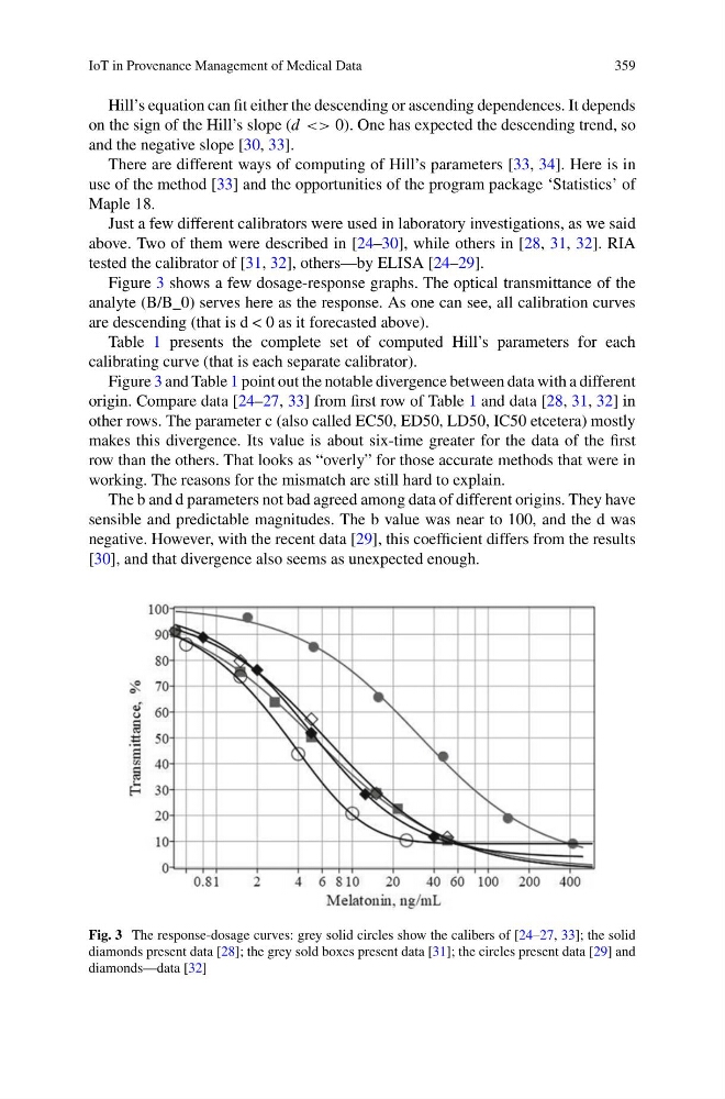
Figure 3 shows a few dosage-response graphs. The optical transmittance of the
analyte (B/B_0) serves here as the response. As one can see, all calibration curves
are descending (that is d < 0 as it forecasted above).
Table 1 presents the complete set of computed Hill’s parameters for each
calibrating curve (that is each separate calibrator).
Figure 3 and Table 1 point out the notable divergence between data with a different
origin. Compare data [24–27, 33] from first row of Table 1 and data [28, 31, 32] in
other rows. The parameter c (also called EC50, ED50, LD50, IC50 etcetera) mostly
makes this divergence. Its value is about six-time greater for the data of the first
row than the others. That looks as “overly” for those accurate methods that were in
working. The reasons for the mismatch are still hard to explain.
The b and d parameters not bad agreed among data of different origins. They have
sensible and predictable magnitudes. The b value was near to 100, and the d was
negative. However, with the recent data [29], this coefficient differs from the results
[30], and that divergence also seems as unexpected enough.
Fig. 3 The response-dosage curves: grey solid circles show the calibers of [24–27, 33]; the solid
diamonds present data [28]; the grey sold boxes present data [31]; the circles present data [29] and
diamonds—data [32]
359
Hill’s equation can fit either the descending or ascending dependences. It depends
on the sign of the Hill’s slope (d <> 0). One has expected the descending trend, so
and the negative slope [30, 33].
There are different ways of computing of Hill’s parameters [33, 34]. Here is in
use of the method [33] and the opportunities of the program package ‘Statistics’ of
Maple 18.
Just a few different calibrators were used in laboratory investigations, as we said
above. Two of them were described in [24–30], while others in [28, 31, 32]. RIA
tested the calibrator of [31, 32], others—by ELISA [24–29].
Figure 3 shows a few dosage-response graphs. The optical transmittance of the
analyte (B/B_0) serves here as the response. As one can see, all calibration curves
are descending (that is d < 0 as it forecasted above).
Table 1 presents the complete set of computed Hill’s parameters for each
calibrating curve (that is each separate calibrator).
Figure 3 and Table 1 point out the notable divergence between data with a different
origin. Compare data [24–27, 33] from first row of Table 1 and data [28, 31, 32] in
other rows. The parameter c (also called EC50, ED50, LD50, IC50 etcetera) mostly
makes this divergence. Its value is about six-time greater for the data of the first
row than the others. That looks as “overly” for those accurate methods that were in
working. The reasons for the mismatch are still hard to explain.
The b and d parameters not bad agreed among data of different origins. They have
sensible and predictable magnitudes. The b value was near to 100, and the d was
negative. However, with the recent data [29], this coefficient differs from the results
[30], and that divergence also seems as unexpected enough.
Fig. 3 The response-dosage curves: grey solid circles show the calibers of [24–27, 33]; the solid
diamonds present data [28]; the grey sold boxes present data [31]; the circles present data [29] and
diamonds—data [32]