

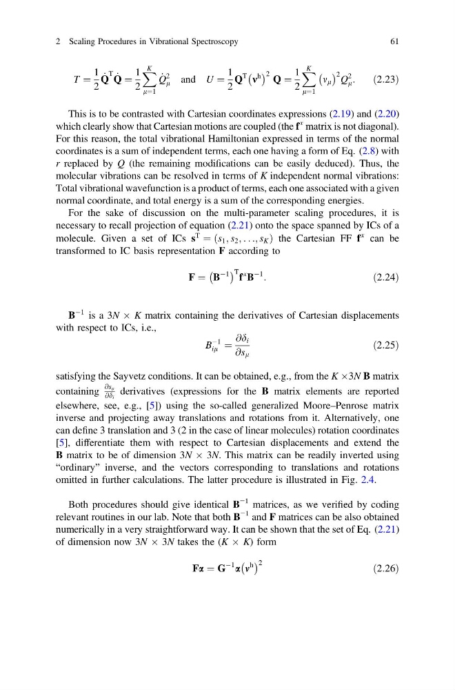
T ¼
1
2
_
Q
T
_
Q ¼
1
2
X K
l¼1
_
Q
2
l and U ¼
1
2
Q
T
m
h
À Á 2 Q ¼
1
2
X K
l¼1
m l
À Á 2 Q
2
l :
ð2:23Þ
This is to be contrasted with Cartesian coordinates expressions (2.19) and (2.20)
which clearly show that Cartesian motions are coupled (the f
x matrix is not diagonal).
For this reason, the total vibrational Hamiltonian expressed in terms of the normal
coordinates is a sum of independent terms, each one having a form of Eq. (2.8) with
r replaced by Q (the remaining modifications can be easily deduced). Thus, the
molecular vibrations can be resolved in terms of K independent normal vibrations:
Total vibrational wavefunction is a product of terms, each one associated with a given
normal coordinate, and total energy is a sum of the corresponding energies.
For the sake of discussion on the multi-parameter scaling procedures, it is
necessary to recall projection of equation (2.21) onto the space spanned by ICs of a
molecule. Given a set of ICs s
T
¼ s 1 ; s 2 ; . . .; s K
ð
Þthe Cartesian FF f
x can be
transformed to IC basis representation F according to
F ¼ B
À1
À
Á T f
x B
À1
:
ð2:24Þ
B
À1 is a 3N Â K matrix containing the derivatives of Cartesian displacements
with respect to ICs, i.e.,
B
À1
il ¼
@d i
@s l
ð2:25Þ
satisfying the Sayvetz conditions. It can be obtained, e.g., from the K Â3N B matrix
containing
@s l
@d i
derivatives (expressions for the B matrix elements are reported
elsewhere, see, e.g., [5]) using the so-called generalized Moore–Penrose matrix
inverse and projecting away translations and rotations from it. Alternatively, one
can define 3 translation and 3 (2 in the case of linear molecules) rotation coordinates
[5], differentiate them with respect to Cartesian displacements and extend the
B matrix to be of dimension 3N Â 3N. This matrix can be readily inverted using
“ordinary” inverse, and the vectors corresponding to translations and rotations
omitted in further calculations. The latter procedure is illustrated in Fig. 2.4.
Both procedures should give identical B
−1 matrices, as we verified by coding
relevant routines in our lab. Note that both B
−1 and F matrices can be also obtained
numerically in a very straightforward way. It can be shown that the set of Eq. (2.21)
of dimension now 3N Â 3N takes the (K Â K) form
Fa ¼ G
À1 a m
h
À Á 2
ð2:26Þ
2 Scaling Procedures in Vibrational Spectroscopy
61
1
2
_
Q
T
_
Q ¼
1
2
X K
l¼1
_
Q
2
l and U ¼
1
2
Q
T
m
h
À Á 2 Q ¼
1
2
X K
l¼1
m l
À Á 2 Q
2
l :
ð2:23Þ
This is to be contrasted with Cartesian coordinates expressions (2.19) and (2.20)
which clearly show that Cartesian motions are coupled (the f
x matrix is not diagonal).
For this reason, the total vibrational Hamiltonian expressed in terms of the normal
coordinates is a sum of independent terms, each one having a form of Eq. (2.8) with
r replaced by Q (the remaining modifications can be easily deduced). Thus, the
molecular vibrations can be resolved in terms of K independent normal vibrations:
Total vibrational wavefunction is a product of terms, each one associated with a given
normal coordinate, and total energy is a sum of the corresponding energies.
For the sake of discussion on the multi-parameter scaling procedures, it is
necessary to recall projection of equation (2.21) onto the space spanned by ICs of a
molecule. Given a set of ICs s
T
¼ s 1 ; s 2 ; . . .; s K
ð
Þthe Cartesian FF f
x can be
transformed to IC basis representation F according to
F ¼ B
À1
À
Á T f
x B
À1
:
ð2:24Þ
B
À1 is a 3N Â K matrix containing the derivatives of Cartesian displacements
with respect to ICs, i.e.,
B
À1
il ¼
@d i
@s l
ð2:25Þ
satisfying the Sayvetz conditions. It can be obtained, e.g., from the K Â3N B matrix
containing
@s l
@d i
derivatives (expressions for the B matrix elements are reported
elsewhere, see, e.g., [5]) using the so-called generalized Moore–Penrose matrix
inverse and projecting away translations and rotations from it. Alternatively, one
can define 3 translation and 3 (2 in the case of linear molecules) rotation coordinates
[5], differentiate them with respect to Cartesian displacements and extend the
B matrix to be of dimension 3N Â 3N. This matrix can be readily inverted using
“ordinary” inverse, and the vectors corresponding to translations and rotations
omitted in further calculations. The latter procedure is illustrated in Fig. 2.4.
Both procedures should give identical B
−1 matrices, as we verified by coding
relevant routines in our lab. Note that both B
−1 and F matrices can be also obtained
numerically in a very straightforward way. It can be shown that the set of Eq. (2.21)
of dimension now 3N Â 3N takes the (K Â K) form
Fa ¼ G
À1 a m
h
À Á 2
ð2:26Þ
2 Scaling Procedures in Vibrational Spectroscopy
61