

where G
À1
¼ B
À1
À
Á T MB
À1 is the so-called mass tensor which is multidimensional
generalization of a reduced mass ðT ¼
1
2
_
s
T G
À1
_
sÞ and a is a transformation matrix
between internal and normal coordinates
s ¼ aQ for the
00 Q part
00 of Q:
ð2:27Þ
In addition, we have L ¼ B
À1
a and
U ¼
1
2
s
T Fs:
ð2:28Þ
In the potential energy expression s denotes deviations of internal coordinates
from their equilibrium values s À s e
ð
Þ, for simplicity. There are some advantages of
using Eq. (2.26) instead of (2.21) in particular, when a new QC method has to be
tested for the prediction of harmonic frequencies of small molecules. Apparently,
much fewer FCs need to be calculated numerically by central differences on energy,
which is always coded first prior to coding analytic gradient and hessian. Note that
Eq. (2.26) is a generalization of Eq. (2.10) as it reduces to the latter one in
one-dimensional case with l ¼ G
À1
11 .
Equations (2.21) and (2.26) provide harmonic vibrational frequencies along with
the atomic Cartesian/internal displacement amplitudes (L/a matrices), the latter
ones being used in the animation of normal modes by graphical interfaces to various
QC packages.
2.3 Scaling Procedures
Theoretical prediction of the vibrational spectra, i.e., calculations of the harmonic
frequencies, became affordable in the end of 1960s [6] when nuclear gradient
formulas become available, initially at the HF computational level with small basis
sets. Numerical differentiation was used to obtain the FC matrix. Somewhat later it
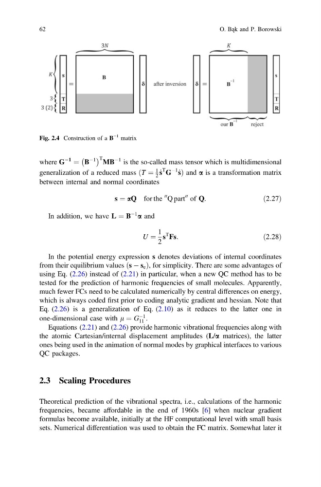
Fig. 2.4 Construction of a B
−1 matrix
62
O. Bąk and P. Borowski
À1
¼ B
À1
À
Á T MB
À1 is the so-called mass tensor which is multidimensional
generalization of a reduced mass ðT ¼
1
2
_
s
T G
À1
_
sÞ and a is a transformation matrix
between internal and normal coordinates
s ¼ aQ for the
00 Q part
00 of Q:
ð2:27Þ
In addition, we have L ¼ B
À1
a and
U ¼
1
2
s
T Fs:
ð2:28Þ
In the potential energy expression s denotes deviations of internal coordinates
from their equilibrium values s À s e
ð
Þ, for simplicity. There are some advantages of
using Eq. (2.26) instead of (2.21) in particular, when a new QC method has to be
tested for the prediction of harmonic frequencies of small molecules. Apparently,
much fewer FCs need to be calculated numerically by central differences on energy,
which is always coded first prior to coding analytic gradient and hessian. Note that
Eq. (2.26) is a generalization of Eq. (2.10) as it reduces to the latter one in
one-dimensional case with l ¼ G
À1
11 .
Equations (2.21) and (2.26) provide harmonic vibrational frequencies along with
the atomic Cartesian/internal displacement amplitudes (L/a matrices), the latter
ones being used in the animation of normal modes by graphical interfaces to various
QC packages.
2.3 Scaling Procedures
Theoretical prediction of the vibrational spectra, i.e., calculations of the harmonic
frequencies, became affordable in the end of 1960s [6] when nuclear gradient
formulas become available, initially at the HF computational level with small basis
sets. Numerical differentiation was used to obtain the FC matrix. Somewhat later it
Fig. 2.4 Construction of a B
−1 matrix
62
O. Bąk and P. Borowski