

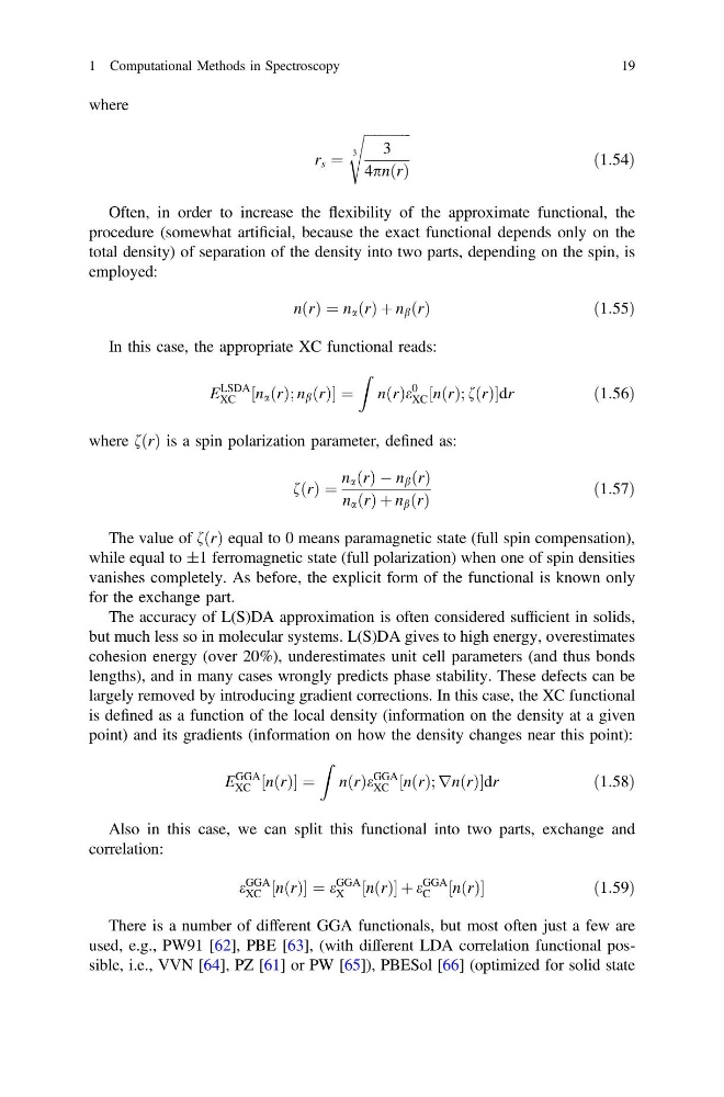
where
r s ¼
ffiffiffiffiffiffiffiffiffiffiffiffiffi ffi
3
4pn r
ð Þ
3
s
ð1:54Þ
Often, in order to increase the flexibility of the approximate functional, the
procedure (somewhat artificial, because the exact functional depends only on the
total density) of separation of the density into two parts, depending on the spin, is
employed:
nðrÞ ¼ n a ðrÞ þ n b ðrÞ
ð 1:55Þ
In this case, the appropriate XC functional reads:
E
LSDA
XC ½n a ðrÞ; n b ðrÞ ¼
Z
nðrÞe
0
XC ½nðrÞ; fðrÞdr
ð1:56Þ
where fðrÞ is a spin polarization parameter, defined as:
fðrÞ ¼
n a ðrÞ À n b ðrÞ
n a ðrÞ þ n b ðrÞ
ð1:57Þ
The value of fðrÞ equal to 0 means paramagnetic state (full spin compensation),
while equal to ±1 ferromagnetic state (full polarization) when one of spin densities
vanishes completely. As before, the explicit form of the functional is known only
for the exchange part.
The accuracy of L(S)DA approximation is often considered sufficient in solids,
but much less so in molecular systems. L(S)DA gives to high energy, overestimates
cohesion energy (over 20%), underestimates unit cell parameters (and thus bonds
lengths), and in many cases wrongly predicts phase stability. These defects can be
largely removed by introducing gradient corrections. In this case, the XC functional
is defined as a function of the local density (information on the density at a given
point) and its gradients (information on how the density changes near this point):
E
GGA
XC ½nðrÞ ¼
Z
nðrÞe
GGA
XC ½nðrÞ; rnðrÞdr
ð1:58Þ
Also in this case, we can split this functional into two parts, exchange and
correlation:
e
GGA
XC ½nðrÞ ¼ e
GGA
X
½nðrÞ þ e
GGA
C
½nðrÞ
ð1:59Þ
There is a number of different GGA functionals, but most often just a few are
used, e.g., PW91 [62], PBE [63], (with different LDA correlation functional possible, i.e., VVN [64], PZ [61] or PW [65]), PBESol [66] (optimized for solid state
1 Computational Methods in Spectroscopy
19
r s ¼
ffiffiffiffiffiffiffiffiffiffiffiffiffi ffi
3
4pn r
ð Þ
3
s
ð1:54Þ
Often, in order to increase the flexibility of the approximate functional, the
procedure (somewhat artificial, because the exact functional depends only on the
total density) of separation of the density into two parts, depending on the spin, is
employed:
nðrÞ ¼ n a ðrÞ þ n b ðrÞ
ð 1:55Þ
In this case, the appropriate XC functional reads:
E
LSDA
XC ½n a ðrÞ; n b ðrÞ ¼
Z
nðrÞe
0
XC ½nðrÞ; fðrÞdr
ð1:56Þ
where fðrÞ is a spin polarization parameter, defined as:
fðrÞ ¼
n a ðrÞ À n b ðrÞ
n a ðrÞ þ n b ðrÞ
ð1:57Þ
The value of fðrÞ equal to 0 means paramagnetic state (full spin compensation),
while equal to ±1 ferromagnetic state (full polarization) when one of spin densities
vanishes completely. As before, the explicit form of the functional is known only
for the exchange part.
The accuracy of L(S)DA approximation is often considered sufficient in solids,
but much less so in molecular systems. L(S)DA gives to high energy, overestimates
cohesion energy (over 20%), underestimates unit cell parameters (and thus bonds
lengths), and in many cases wrongly predicts phase stability. These defects can be
largely removed by introducing gradient corrections. In this case, the XC functional
is defined as a function of the local density (information on the density at a given
point) and its gradients (information on how the density changes near this point):
E
GGA
XC ½nðrÞ ¼
Z
nðrÞe
GGA
XC ½nðrÞ; rnðrÞdr
ð1:58Þ
Also in this case, we can split this functional into two parts, exchange and
correlation:
e
GGA
XC ½nðrÞ ¼ e
GGA
X
½nðrÞ þ e
GGA
C
½nðrÞ
ð1:59Þ
There is a number of different GGA functionals, but most often just a few are
used, e.g., PW91 [62], PBE [63], (with different LDA correlation functional possible, i.e., VVN [64], PZ [61] or PW [65]), PBESol [66] (optimized for solid state
1 Computational Methods in Spectroscopy
19