

94
6 Applications
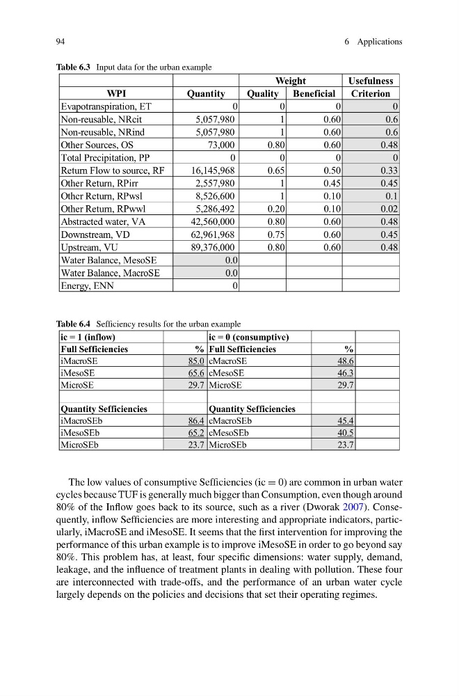
Table 6.3 Input data for the urban example
Usefulness
WPI
Quantity
Quality Beneficial
Criterion
Evapotranspiration, ET
0
0
0
0
Non-reusable, NRcit
5,057,980
1
0.60
0.6
Non-reusable, NRind
5,057,980
1
0.60
0.6
Other Sources, OS
73,000
0.80
0.60
0.48
Total Precipitation, PP
0
0
0
0
Return Flow to source, RF
16,145,968
0.65
0.50
0.33
Other Return, RPirr
2,557,980
1
0.45
0.45
Other Return, RPwsl
8,526,600
1
0.10
0.1
Other Return, RPwwl
5,286,492
0.20
0.10
0.02
Abstracted water, VA
42,560,000
0.80
0.60
0.48
Downstream, VD
62,961,968
0.75
0.60
0.45
Upstream, VU
89,376,000
0.80
0.60
0.48
Water Balance, MesoSE
0.0
Water Balance, MacroSE
0.0
Energy, ENN
0
Weight
Table 6.4 Sefficiency results for the urban example
ic = 1 (inflow)
ic = 0 (consumptive)
Full Sefficiencies
% Full Sefficiencies
%
iMacroSE
85.0 cMacroSE
48.6
iMesoSE
65.6 cMesoSE
46.3
MicroSE
29.7 MicroSE
29.7
Quantity Sefficiencies
Quantity Sefficiencies
iMacroSEb
86.4 cMacroSEb
45.4
iMesoSEb
65.2 cMesoSEb
40.5
MicroSEb
23.7 MicroSEb
23.7
The low values of consumptive Sefficiencies (ic = 0) are common in urban water
cycles because TUF is generally much bigger than Consumption, even though around
80% of the Inflow goes back to its source, such as a river (Dworak 2007). Consequently, inflow Sefficiencies are more interesting and appropriate indicators, particularly, iMacroSE and iMesoSE. It seems that the first intervention for improving the
performance of this urban example is to improve iMesoSE in order to go beyond say
80%. This problem has, at least, four specific dimensions: water supply, demand,
leakage, and the influence of treatment plants in dealing with pollution. These four
are interconnected with trade-offs, and the performance of an urban water cycle
largely depends on the policies and decisions that set their operating regimes.
6 Applications
Table 6.3 Input data for the urban example
Usefulness
WPI
Quantity
Quality Beneficial
Criterion
Evapotranspiration, ET
0
0
0
0
Non-reusable, NRcit
5,057,980
1
0.60
0.6
Non-reusable, NRind
5,057,980
1
0.60
0.6
Other Sources, OS
73,000
0.80
0.60
0.48
Total Precipitation, PP
0
0
0
0
Return Flow to source, RF
16,145,968
0.65
0.50
0.33
Other Return, RPirr
2,557,980
1
0.45
0.45
Other Return, RPwsl
8,526,600
1
0.10
0.1
Other Return, RPwwl
5,286,492
0.20
0.10
0.02
Abstracted water, VA
42,560,000
0.80
0.60
0.48
Downstream, VD
62,961,968
0.75
0.60
0.45
Upstream, VU
89,376,000
0.80
0.60
0.48
Water Balance, MesoSE
0.0
Water Balance, MacroSE
0.0
Energy, ENN
0
Weight
Table 6.4 Sefficiency results for the urban example
ic = 1 (inflow)
ic = 0 (consumptive)
Full Sefficiencies
% Full Sefficiencies
%
iMacroSE
85.0 cMacroSE
48.6
iMesoSE
65.6 cMesoSE
46.3
MicroSE
29.7 MicroSE
29.7
Quantity Sefficiencies
Quantity Sefficiencies
iMacroSEb
86.4 cMacroSEb
45.4
iMesoSEb
65.2 cMesoSEb
40.5
MicroSEb
23.7 MicroSEb
23.7
The low values of consumptive Sefficiencies (ic = 0) are common in urban water
cycles because TUF is generally much bigger than Consumption, even though around
80% of the Inflow goes back to its source, such as a river (Dworak 2007). Consequently, inflow Sefficiencies are more interesting and appropriate indicators, particularly, iMacroSE and iMesoSE. It seems that the first intervention for improving the
performance of this urban example is to improve iMesoSE in order to go beyond say
80%. This problem has, at least, four specific dimensions: water supply, demand,
leakage, and the influence of treatment plants in dealing with pollution. These four
are interconnected with trade-offs, and the performance of an urban water cycle
largely depends on the policies and decisions that set their operating regimes.