

13 Assessment of Hydrological Impacts …
289
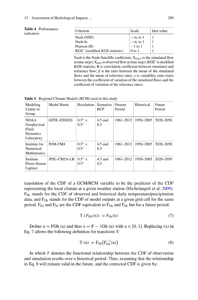
Table 4 Performance
indicators
Criterion
Scale
Idea value
Nash (NSE)
Nash-ln
Pearson (R)
KGE’ (modified KGE-statistic)
−∞ to 1
−∞ to 1
−1 to 1
0 to 1
1
1
1
1
Nash is the Nash-Sutcliffe coefficient; X sim,t is the simulated flow
at time step t; X ref,t is observed flow at time step t; KGE’ is modified
KGE-statistic; R is correlation coefficient between simulated and
reference flow; β is the ratio between the mean of the simulated
flows and the mean of reference ones; γ is variability ratio (ratio
between the coefficient of variation of the simulated flows and the
coefficient of variation of the reference ones)
Table 5 Regional Climate Models (RCM) used in this study
Modeling
Center or
Group
Model Name
Resolution Scenarios
RCP
Present
Period
Historical Future
Period
NOAA
Geophysical
Fluid
Dynamics
Laboratory
GFDL-ESM2G 0.5° ×
0.5°
4.5 and
8.5
1961–2012 1950–2005 2020–2050
Institute for
Numerical
Mathematics
INM-CM4
0.5° ×
0.5°
4.5 and
8.5
1961–2012 1950–2005 2020–2050
Institute
Pierre-Simon
Laplace
IPSL-CM5A-LR 0.5° ×
0.5°
4.5 and
8.5
1961–2012 1950–2005 2020–2050
translation of the CDF of a GCM/RCM variable to be the predictor of the CDF
representing the local climate at a given weather station (Michelangeli et al. 2009).
F Sh stands for the CDF of observed and historical daily temperature/precipitation
data, and F Gh stands for the CDF of model outputs at a given grid cell for the same
period. F Gf and F Sf are the CDF equivalent to F Gh and F Sh but for a future period.
T (F Gh (x)) = F Sh (x)
(7)
Define u = FGh (x) and thus x = F − 1Gh (u) with u ∈ [0, 1]. Replacing (x) in
Eq. 7 allows the following definition for transform T:
T (u) = F Sh
F
− 1
Gh (u)
(8)
In which T denotes the functional relationship between the CDF of observation
and simulation results over a historical period. Thus, assuming that the relationship
in Eq. 8 will remain valid in the future, and the corrected CDF is given by:
289
Table 4 Performance
indicators
Criterion
Scale
Idea value
Nash (NSE)
Nash-ln
Pearson (R)
KGE’ (modified KGE-statistic)
−∞ to 1
−∞ to 1
−1 to 1
0 to 1
1
1
1
1
Nash is the Nash-Sutcliffe coefficient; X sim,t is the simulated flow
at time step t; X ref,t is observed flow at time step t; KGE’ is modified
KGE-statistic; R is correlation coefficient between simulated and
reference flow; β is the ratio between the mean of the simulated
flows and the mean of reference ones; γ is variability ratio (ratio
between the coefficient of variation of the simulated flows and the
coefficient of variation of the reference ones)
Table 5 Regional Climate Models (RCM) used in this study
Modeling
Center or
Group
Model Name
Resolution Scenarios
RCP
Present
Period
Historical Future
Period
NOAA
Geophysical
Fluid
Dynamics
Laboratory
GFDL-ESM2G 0.5° ×
0.5°
4.5 and
8.5
1961–2012 1950–2005 2020–2050
Institute for
Numerical
Mathematics
INM-CM4
0.5° ×
0.5°
4.5 and
8.5
1961–2012 1950–2005 2020–2050
Institute
Pierre-Simon
Laplace
IPSL-CM5A-LR 0.5° ×
0.5°
4.5 and
8.5
1961–2012 1950–2005 2020–2050
translation of the CDF of a GCM/RCM variable to be the predictor of the CDF
representing the local climate at a given weather station (Michelangeli et al. 2009).
F Sh stands for the CDF of observed and historical daily temperature/precipitation
data, and F Gh stands for the CDF of model outputs at a given grid cell for the same
period. F Gf and F Sf are the CDF equivalent to F Gh and F Sh but for a future period.
T (F Gh (x)) = F Sh (x)
(7)
Define u = FGh (x) and thus x = F − 1Gh (u) with u ∈ [0, 1]. Replacing (x) in
Eq. 7 allows the following definition for transform T:
T (u) = F Sh
F
− 1
Gh (u)
(8)
In which T denotes the functional relationship between the CDF of observation
and simulation results over a historical period. Thus, assuming that the relationship
in Eq. 8 will remain valid in the future, and the corrected CDF is given by: