

288
I. Thiaw et al.
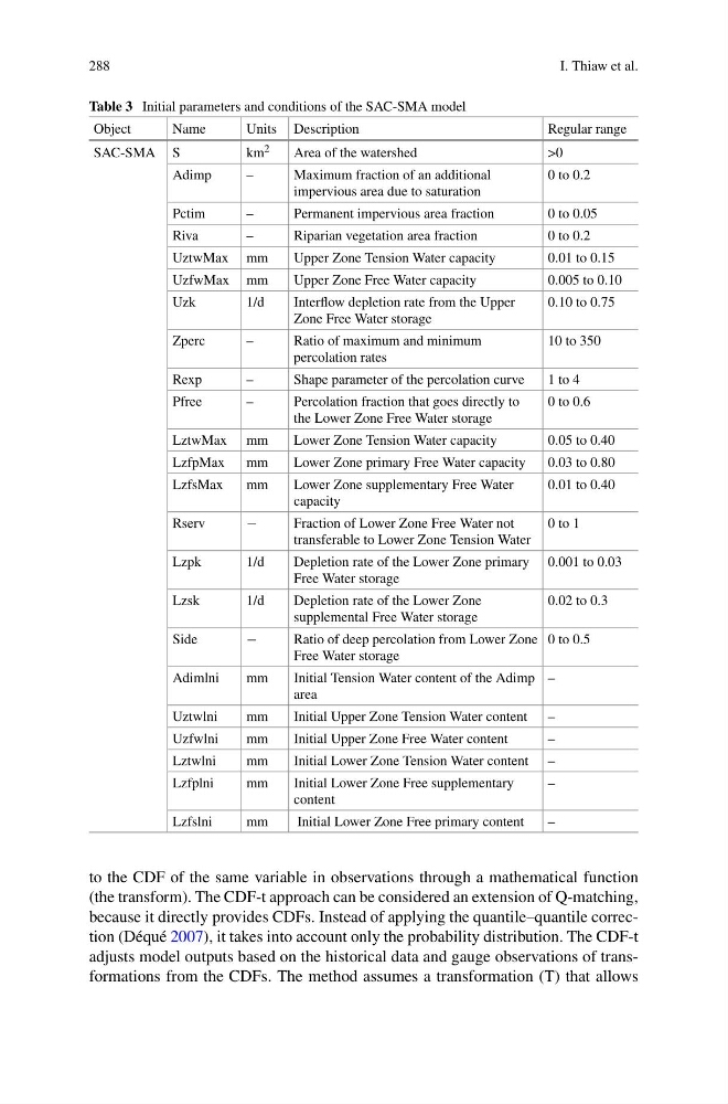
Table 3 Initial parameters and conditions of the SAC-SMA model
Object
Name
Units Description
Regular range
SAC-SMA S
km 2
Area of the watershed
>0
Adimp
–
Maximum fraction of an additional
impervious area due to saturation
0 to 0.2
Pctim
–
Permanent impervious area fraction
0 to 0.05
Riva
–
Riparian vegetation area fraction
0 to 0.2
UztwMax mm
Upper Zone Tension Water capacity
0.01 to 0.15
UzfwMax mm
Upper Zone Free Water capacity
0.005 to 0.10
Uzk
1/d
Interflow depletion rate from the Upper
Zone Free Water storage
0.10 to 0.75
Zperc
–
Ratio of maximum and minimum
percolation rates
10 to 350
Rexp
–
Shape parameter of the percolation curve
1 to 4
Pfree
–
Percolation fraction that goes directly to
the Lower Zone Free Water storage
0 to 0.6
LztwMax mm
Lower Zone Tension Water capacity
0.05 to 0.40
LzfpMax
mm
Lower Zone primary Free Water capacity
0.03 to 0.80
LzfsMax
mm
Lower Zone supplementary Free Water
capacity
0.01 to 0.40
Rserv
−
Fraction of Lower Zone Free Water not
transferable to Lower Zone Tension Water
0 to 1
Lzpk
1/d
Depletion rate of the Lower Zone primary
Free Water storage
0.001 to 0.03
Lzsk
1/d
Depletion rate of the Lower Zone
supplemental Free Water storage
0.02 to 0.3
Side
−
Ratio of deep percolation from Lower Zone
Free Water storage
0 to 0.5
Adimlni
mm
Initial Tension Water content of the Adimp
area
–
Uztwlni
mm
Initial Upper Zone Tension Water content –
Uzfwlni
mm
Initial Upper Zone Free Water content
–
Lztwlni
mm
Initial Lower Zone Tension Water content –
Lzfplni
mm
Initial Lower Zone Free supplementary
content
–
Lzfslni
mm
Initial Lower Zone Free primary content
–
to the CDF of the same variable in observations through a mathematical function
(the transform). The CDF-t approach can be considered an extension of Q-matching,
because it directly provides CDFs. Instead of applying the quantile–quantile correction (Déqué 2007), it takes into account only the probability distribution. The CDF-t
adjusts model outputs based on the historical data and gauge observations of transformations from the CDFs. The method assumes a transformation (T) that allows
I. Thiaw et al.
Table 3 Initial parameters and conditions of the SAC-SMA model
Object
Name
Units Description
Regular range
SAC-SMA S
km 2
Area of the watershed
>0
Adimp
–
Maximum fraction of an additional
impervious area due to saturation
0 to 0.2
Pctim
–
Permanent impervious area fraction
0 to 0.05
Riva
–
Riparian vegetation area fraction
0 to 0.2
UztwMax mm
Upper Zone Tension Water capacity
0.01 to 0.15
UzfwMax mm
Upper Zone Free Water capacity
0.005 to 0.10
Uzk
1/d
Interflow depletion rate from the Upper
Zone Free Water storage
0.10 to 0.75
Zperc
–
Ratio of maximum and minimum
percolation rates
10 to 350
Rexp
–
Shape parameter of the percolation curve
1 to 4
Pfree
–
Percolation fraction that goes directly to
the Lower Zone Free Water storage
0 to 0.6
LztwMax mm
Lower Zone Tension Water capacity
0.05 to 0.40
LzfpMax
mm
Lower Zone primary Free Water capacity
0.03 to 0.80
LzfsMax
mm
Lower Zone supplementary Free Water
capacity
0.01 to 0.40
Rserv
−
Fraction of Lower Zone Free Water not
transferable to Lower Zone Tension Water
0 to 1
Lzpk
1/d
Depletion rate of the Lower Zone primary
Free Water storage
0.001 to 0.03
Lzsk
1/d
Depletion rate of the Lower Zone
supplemental Free Water storage
0.02 to 0.3
Side
−
Ratio of deep percolation from Lower Zone
Free Water storage
0 to 0.5
Adimlni
mm
Initial Tension Water content of the Adimp
area
–
Uztwlni
mm
Initial Upper Zone Tension Water content –
Uzfwlni
mm
Initial Upper Zone Free Water content
–
Lztwlni
mm
Initial Lower Zone Tension Water content –
Lzfplni
mm
Initial Lower Zone Free supplementary
content
–
Lzfslni
mm
Initial Lower Zone Free primary content
–
to the CDF of the same variable in observations through a mathematical function
(the transform). The CDF-t approach can be considered an extension of Q-matching,
because it directly provides CDFs. Instead of applying the quantile–quantile correction (Déqué 2007), it takes into account only the probability distribution. The CDF-t
adjusts model outputs based on the historical data and gauge observations of transformations from the CDFs. The method assumes a transformation (T) that allows