

22.5.1 Without Project State
In the without project state, we can imagine how a certain parameter will change
with time. This parameter will, of course, depend on our field of interest. For
example, in agriculture we might be thinking of crop yield, in education it might
be student performance, in the transport sector it might be number of vehicles in
good condition, travel time, number of passengers transported, etc.
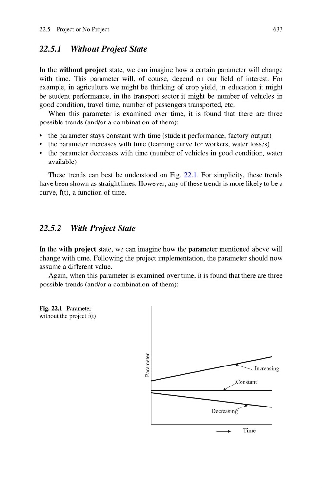
When this parameter is examined over time, it is found that there are three
possible trends (and/or a combination of them):
• the parameter stays constant with time (student performance, factory output)
• the parameter increases with time (learning curve for workers, water losses)
• the parameter decreases with time (number of vehicles in good condition, water
available)
These trends can best be understood on Fig. 22.1. For simplicity, these trends
have been shown as straight lines. However, any of these trends is more likely to be a
curve, f(t), a function of time.
22.5.2 With Project State
In the with project state, we can imagine how the parameter mentioned above will
change with time. Following the project implementation, the parameter should now
assume a different value.
Again, when this parameter is examined over time, it is found that there are three
possible trends (and/or a combination of them):
Parameter
Increasing
Constant
Decreasing
Time
Fig. 22.1 Parameter
without the project f(t)
22.5 Project or No Project
633