

expected incremental profit ¼ p IP
ð Þ
¼ Rs:0:8 Â 5 ¼ Rs:4,
expected incremental loss ¼ 1 À p
ð
Þ IL
ð Þ ¼ Rs:0:2 Â 2 ¼ Rs:4:
For 56 litres of stock level, the expected incremental loss will be more than the
expected incremental gain.
The use of incremental analysis yields the same solution as provided by the EMV
and EOL approaches. However, the computational effort required in this approach is
much less.
16.6.6 Maximum Likelihood Criterion
According to this criterion, the decision maker just chooses the event (state of nature)
that has the highest occurrence probability and then picks the decision alternative
which produces the highest payoff in that state of nature. For instance, referring to
Table 16.20a of Example 16.6, the ice-cream retailer would choose the demand level
of 17 cups that corresponds to the highest probability of 0.40 and having selected
that, would decide in favour of stock action of 17 cups since it results in the largest
conditional profit of Rs. 510 in that state of nature.
This decision criterion produces valid results when the probability of one state of
nature is significantly higher than any other and when the conditional values do not
differ too much. This criterion, however, may result in serious errors when there are
a large number of states of nature, with each of them having associated probabilities
which are small and nearly equal.
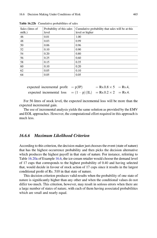
Table 16.22b Cumulative probabilities of sales
Sales (litres of
milk.)
Probability of this sales
level
Cumulative probability that sales will be at this
level or higher
46
0.01
1.00
48
0.03
0.99
50
0.06
0.96
52
0.10
0.90
54
0.20
0.80
56
0.25
0.60
58
0.15
0.35
60
0.10
0.20
62
0.05
0.10
64
0.05
0.05
16.6 Decision Making Under Conditions of Risk
465
ð Þ
¼ Rs:0:8 Â 5 ¼ Rs:4,
expected incremental loss ¼ 1 À p
ð
Þ IL
ð Þ ¼ Rs:0:2 Â 2 ¼ Rs:4:
For 56 litres of stock level, the expected incremental loss will be more than the
expected incremental gain.
The use of incremental analysis yields the same solution as provided by the EMV
and EOL approaches. However, the computational effort required in this approach is
much less.
16.6.6 Maximum Likelihood Criterion
According to this criterion, the decision maker just chooses the event (state of nature)
that has the highest occurrence probability and then picks the decision alternative
which produces the highest payoff in that state of nature. For instance, referring to
Table 16.20a of Example 16.6, the ice-cream retailer would choose the demand level
of 17 cups that corresponds to the highest probability of 0.40 and having selected
that, would decide in favour of stock action of 17 cups since it results in the largest
conditional profit of Rs. 510 in that state of nature.
This decision criterion produces valid results when the probability of one state of
nature is significantly higher than any other and when the conditional values do not
differ too much. This criterion, however, may result in serious errors when there are
a large number of states of nature, with each of them having associated probabilities
which are small and nearly equal.
Table 16.22b Cumulative probabilities of sales
Sales (litres of
milk.)
Probability of this sales
level
Cumulative probability that sales will be at this
level or higher
46
0.01
1.00
48
0.03
0.99
50
0.06
0.96
52
0.10
0.90
54
0.20
0.80
56
0.25
0.60
58
0.15
0.35
60
0.10
0.20
62
0.05
0.10
64
0.05
0.05
16.6 Decision Making Under Conditions of Risk
465