

16.6.7 Expected Value Criterion for Continuously Distributed
Random Variables
The situations considered up to now involved discrete random variables. Many real
situations, however, are concerned with continuously distributed random variables.
The expected value criterion discussed above can be applied for such situations also.
Example 16.8
A vegetable trader purchases tomatoes for Rs. 450 a box and sells them at
Rs. 800 per box. If unsold on the first day, the box has a salvage value of Rs. 150.
Past records have indicated normal distribution for the demand with a daily mean
and standard deviation of 30 and 9 boxes, respectively. How many boxes should he
stock?
Solution
The minimum probability required for the sale of at least an additional box (unit)
to substantiate the storage of that box is
p ¼
IL
IP þ IL
¼
450 À 150
ð
Þ
800 À 450
ð
Þþ 450 À 150
ð
Þ
¼
300
350 þ 300
¼
300
650
¼ 0:462
This probability value implies that the vegetable trader must be 0.462 sure of
selling at least an additional unit before it would pay him to stock that unit.
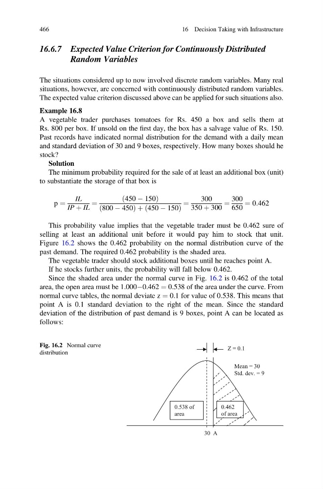
Figure 16.2 shows the 0.462 probability on the normal distribution curve of the
past demand. The required 0.462 probability is the shaded area.
The vegetable trader should stock additional boxes until he reaches point A.
If he stocks further units, the probability will fall below 0.462.
Since the shaded area under the normal curve in Fig. 16.2 is 0.462 of the total
area, the open area must be 1.000À0.462 ¼ 0.538 of the area under the curve. From
normal curve tables, the normal deviate z ¼ 0.1 for value of 0.538. This means that
point A is 0.1 standard deviation to the right of the mean. Since the standard
deviation of the distribution of past demand is 9 boxes, point A can be located as
follows:
Z = 0.1
Mean = 30
Std. dev. = 9
0.538 of
area
0.462
of area
30 A
Fig. 16.2 Normal curve
distribution
466
16 Decision Taking with Infrastructure
Random Variables
The situations considered up to now involved discrete random variables. Many real
situations, however, are concerned with continuously distributed random variables.
The expected value criterion discussed above can be applied for such situations also.
Example 16.8
A vegetable trader purchases tomatoes for Rs. 450 a box and sells them at
Rs. 800 per box. If unsold on the first day, the box has a salvage value of Rs. 150.
Past records have indicated normal distribution for the demand with a daily mean
and standard deviation of 30 and 9 boxes, respectively. How many boxes should he
stock?
Solution
The minimum probability required for the sale of at least an additional box (unit)
to substantiate the storage of that box is
p ¼
IL
IP þ IL
¼
450 À 150
ð
Þ
800 À 450
ð
Þþ 450 À 150
ð
Þ
¼
300
350 þ 300
¼
300
650
¼ 0:462
This probability value implies that the vegetable trader must be 0.462 sure of
selling at least an additional unit before it would pay him to stock that unit.
Figure 16.2 shows the 0.462 probability on the normal distribution curve of the
past demand. The required 0.462 probability is the shaded area.
The vegetable trader should stock additional boxes until he reaches point A.
If he stocks further units, the probability will fall below 0.462.
Since the shaded area under the normal curve in Fig. 16.2 is 0.462 of the total
area, the open area must be 1.000À0.462 ¼ 0.538 of the area under the curve. From
normal curve tables, the normal deviate z ¼ 0.1 for value of 0.538. This means that
point A is 0.1 standard deviation to the right of the mean. Since the standard
deviation of the distribution of past demand is 9 boxes, point A can be located as
follows:
Z = 0.1
Mean = 30
Std. dev. = 9
0.538 of
area
0.462
of area
30 A
Fig. 16.2 Normal curve
distribution
466
16 Decision Taking with Infrastructure