

conditional profits from Rs. 2000. Likewise, for the demand of 110, 120, 130 and
140 copies, the conditional payoff values for each of these rows can be deducted
from the maxima of that row. The resulting conditional opportunity loss (COL) is
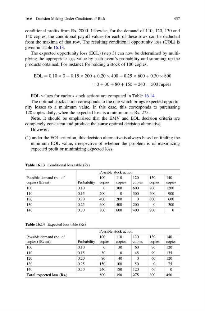
given in Table 16.13.
The expected opportunity loss (EOL) (step 3) can now be determined by multiplying the appropriate loss value by each event’s probability and summing up the
products obtained. For instance for holding a stock of 100 copies,
EOL ¼ 0:10 Â 0 þ 0:15 Â 200 þ 0:20 Â 400 þ 0:25 Â 600 þ 0:30 Â 800
¼ 0 þ 30 þ 80 þ 150 þ 240 ¼ 500 rupees
EOL values for various stock actions are computed in Table 16.14.
The optimal stock action corresponds to the one which brings expected opportunity losses to a minimum value. In this case, this corresponds to purchasing
120 copies daily, when the expected loss is a minimum at Rs. 275.
Note. It should be emphasised that the EMV and EOL decision criteria are
completely consistent and produce the same optimal decision alternative.
However,
(1) under the EOL criterion, this decision alternative is always based on finding the
minimum EOL value, irrespective of whether the problem is of maximizing
expected profit or minimizing expected loss
Table 16.13 Conditional loss table (Rs)
Possible demand (no. of
copies) (Event)
Probability
Possible stock action
100
copies
110
copies
120
copies
130
copies
140
copies
100
0.10
0
300
600
900
1200
110
0.15
200
0
300
600
900
120
0.20
400
200
0
300
600
130
0.25
600
400
200
0
300
140
0.30
800
600
400
200
0
Table 16.14 Expected loss table (Rs)
Possible demand (no. of
copies) (Event)
Probability
Possible stock action
100
copies
110
copies
120
copies
130
copies
140
copies
100
0.10
0
30
60
90
120
110
0.15
30
0
45
90
135
120
0.20
80
40
0
60
120
130
0.25
150
100
50
0
75
140
0.30
240
180
120
60
0
Total expected loss (Rs.)
500
350
275
300
450
16.6 Decision Making Under Conditions of Risk
457
140 copies, the conditional payoff values for each of these rows can be deducted
from the maxima of that row. The resulting conditional opportunity loss (COL) is
given in Table 16.13.
The expected opportunity loss (EOL) (step 3) can now be determined by multiplying the appropriate loss value by each event’s probability and summing up the
products obtained. For instance for holding a stock of 100 copies,
EOL ¼ 0:10 Â 0 þ 0:15 Â 200 þ 0:20 Â 400 þ 0:25 Â 600 þ 0:30 Â 800
¼ 0 þ 30 þ 80 þ 150 þ 240 ¼ 500 rupees
EOL values for various stock actions are computed in Table 16.14.
The optimal stock action corresponds to the one which brings expected opportunity losses to a minimum value. In this case, this corresponds to purchasing
120 copies daily, when the expected loss is a minimum at Rs. 275.
Note. It should be emphasised that the EMV and EOL decision criteria are
completely consistent and produce the same optimal decision alternative.
However,
(1) under the EOL criterion, this decision alternative is always based on finding the
minimum EOL value, irrespective of whether the problem is of maximizing
expected profit or minimizing expected loss
Table 16.13 Conditional loss table (Rs)
Possible demand (no. of
copies) (Event)
Probability
Possible stock action
100
copies
110
copies
120
copies
130
copies
140
copies
100
0.10
0
300
600
900
1200
110
0.15
200
0
300
600
900
120
0.20
400
200
0
300
600
130
0.25
600
400
200
0
300
140
0.30
800
600
400
200
0
Table 16.14 Expected loss table (Rs)
Possible demand (no. of
copies) (Event)
Probability
Possible stock action
100
copies
110
copies
120
copies
130
copies
140
copies
100
0.10
0
30
60
90
120
110
0.15
30
0
45
90
135
120
0.20
80
40
0
60
120
130
0.25
150
100
50
0
75
140
0.30
240
180
120
60
0
Total expected loss (Rs.)
500
350
275
300
450
16.6 Decision Making Under Conditions of Risk
457