

the representative of municipality 1 must then mention how much, if any, he is
willing to increase treatment efficiency in order to achieve a more equitable solution.
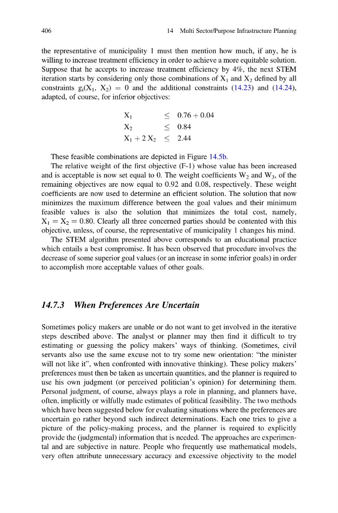
Suppose that he accepts to increase treatment efficiency by 4%, the next STEM
iteration starts by considering only those combinations of X 1 and X 2 defined by all
constraints g i (X 1 , X 2 ) ¼ 0 and the additional constraints (14.23) and (14.24),
adapted, of course, for inferior objectives:
X 1
0:76 þ 0:04
X 2
0:84
X 1 þ 2 X 2
2:44
These feasible combinations are depicted in Figure 14.5b.
The relative weight of the first objective (F-1) whose value has been increased
and is acceptable is now set equal to 0. The weight coefficients W 2 and W 3 , of the
remaining objectives are now equal to 0.92 and 0.08, respectively. These weight
coefficients are now used to determine an efficient solution. The solution that now
minimizes the maximum difference between the goal values and their minimum
feasible values is also the solution that minimizes the total cost, namely,
X 1 ¼ X 2 ¼ 0.80. Clearly all three concerned parties should be contented with this
objective, unless, of course, the representative of municipality 1 changes his mind.
The STEM algorithm presented above corresponds to an educational practice
which entails a best compromise. It has been observed that procedure involves the
decrease of some superior goal values (or an increase in some inferior goals) in order
to accomplish more acceptable values of other goals.
14.7.3 When Preferences Are Uncertain
Sometimes policy makers are unable or do not want to get involved in the iterative
steps described above. The analyst or planner may then find it difficult to try
estimating or guessing the policy makers’ ways of thinking. (Sometimes, civil
servants also use the same excuse not to try some new orientation: “the minister
will not like it”, when confronted with innovative thinking). These policy makers’
preferences must then be taken as uncertain quantities, and the planner is required to
use his own judgment (or perceived politician’s opinion) for determining them.
Personal judgment, of course, always plays a role in planning, and planners have,
often, implicitly or wilfully made estimates of political feasibility. The two methods
which have been suggested below for evaluating situations where the preferences are
uncertain go rather beyond such indirect determinations. Each one tries to give a
picture of the policy-making process, and the planner is required to explicitly
provide the (judgmental) information that is needed. The approaches are experimental and are subjective in nature. People who frequently use mathematical models,
very often attribute unnecessary accuracy and excessive objectivity to the model
406
14 Multi Sector/Purpose Infrastructure Planning
willing to increase treatment efficiency in order to achieve a more equitable solution.
Suppose that he accepts to increase treatment efficiency by 4%, the next STEM
iteration starts by considering only those combinations of X 1 and X 2 defined by all
constraints g i (X 1 , X 2 ) ¼ 0 and the additional constraints (14.23) and (14.24),
adapted, of course, for inferior objectives:
X 1
0:76 þ 0:04
X 2
0:84
X 1 þ 2 X 2
2:44
These feasible combinations are depicted in Figure 14.5b.
The relative weight of the first objective (F-1) whose value has been increased
and is acceptable is now set equal to 0. The weight coefficients W 2 and W 3 , of the
remaining objectives are now equal to 0.92 and 0.08, respectively. These weight
coefficients are now used to determine an efficient solution. The solution that now
minimizes the maximum difference between the goal values and their minimum
feasible values is also the solution that minimizes the total cost, namely,
X 1 ¼ X 2 ¼ 0.80. Clearly all three concerned parties should be contented with this
objective, unless, of course, the representative of municipality 1 changes his mind.
The STEM algorithm presented above corresponds to an educational practice
which entails a best compromise. It has been observed that procedure involves the
decrease of some superior goal values (or an increase in some inferior goals) in order
to accomplish more acceptable values of other goals.
14.7.3 When Preferences Are Uncertain
Sometimes policy makers are unable or do not want to get involved in the iterative
steps described above. The analyst or planner may then find it difficult to try
estimating or guessing the policy makers’ ways of thinking. (Sometimes, civil
servants also use the same excuse not to try some new orientation: “the minister
will not like it”, when confronted with innovative thinking). These policy makers’
preferences must then be taken as uncertain quantities, and the planner is required to
use his own judgment (or perceived politician’s opinion) for determining them.
Personal judgment, of course, always plays a role in planning, and planners have,
often, implicitly or wilfully made estimates of political feasibility. The two methods
which have been suggested below for evaluating situations where the preferences are
uncertain go rather beyond such indirect determinations. Each one tries to give a
picture of the policy-making process, and the planner is required to explicitly
provide the (judgmental) information that is needed. The approaches are experimental and are subjective in nature. People who frequently use mathematical models,
very often attribute unnecessary accuracy and excessive objectivity to the model
406
14 Multi Sector/Purpose Infrastructure Planning