

calculation phase, several distinct decreases between 0 and the maximum acceptable
decrease ΔF
Ã
j of each acceptable objective can be assessed. When the best compromise solution has been identified, the relative weights that would produce this
solution can be calculated a posteriori if required or desired, by the simultaneous
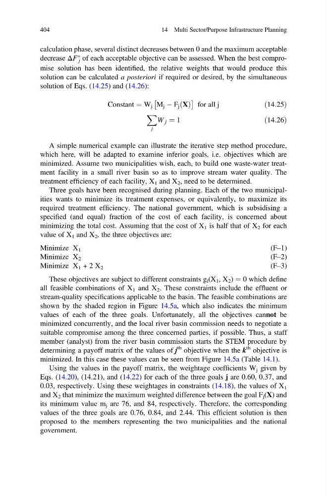
solution of Eqs. (14.25) and (14.26):
Constant ¼ W j M j À F j X
ð Þ
Â
Ã
for all j
ð14:25Þ
X
j
W j ¼ 1
ð14:26Þ
A simple numerical example can illustrate the iterative step method procedure,
which here, will be adapted to examine inferior goals, i.e. objectives which are
minimized. Assume two municipalities wish, each, to build one waste-water treatment facility in a small river basin so as to improve stream water quality. The
treatment efficiency of each facility, X 1 and X 2 , need to be determined.
Three goals have been recognised during planning. Each of the two municipalities wants to minimize its treatment expenses, or equivalently, to maximize its
required treatment efficiency. The national government, which is subsidising a
specified (and equal) fraction of the cost of each facility, is concerned about
minimizing the total cost. Assuming that the cost of X 1 is half that of X 2 for each
value of X 1 and X 2 , the three objectives are:
Minimize X 1
(F–1)
Minimize X 2
(F–2)
Minimize X 1 + 2 X 2
(F–3)
These objectives are subject to different constraints g i (X 1 , X 2 ) ¼ 0 which define
all feasible combinations of X 1 and X 2 . These constraints include the effluent or
stream-quality specifications applicable to the basin. The feasible combinations are
shown by the shaded region in Figure 14.5a, which also indicates the minimum
values of each of the three goals. Unfortunately, all the objectives cannot be
minimized concurrently, and the local river basin commission needs to negotiate a
suitable compromise among the three concerned parties, if possible. Thus, a staff
member (analyst) from the river basin commission starts the STEM procedure by
determining a payoff matrix of the values of j
th objective when the k
th objective is
minimized. In this case these values can be seen from Figure 14.5a (Table 14.1).
Using the values in the payoff matrix, the weightage coefficients W j given by
Eqs. (14.20), (14.21), and (14.22) for each of the three goals j are 0.60, 0.37, and
0.03, respectively. Using these weightages in constraints (14.18), the values of X 1
and X 2 that minimize the maximum weighted difference between the goal F j (X) and
its minimum value m j are 76, and 84, respectively. Therefore, the corresponding
values of the three goals are 0.76, 0.84, and 2.44. This efficient solution is then
proposed to the members representing the two municipalities and the national
government.
404
14 Multi Sector/Purpose Infrastructure Planning
decrease ΔF
Ã
j of each acceptable objective can be assessed. When the best compromise solution has been identified, the relative weights that would produce this
solution can be calculated a posteriori if required or desired, by the simultaneous
solution of Eqs. (14.25) and (14.26):
Constant ¼ W j M j À F j X
ð Þ
Â
Ã
for all j
ð14:25Þ
X
j
W j ¼ 1
ð14:26Þ
A simple numerical example can illustrate the iterative step method procedure,
which here, will be adapted to examine inferior goals, i.e. objectives which are
minimized. Assume two municipalities wish, each, to build one waste-water treatment facility in a small river basin so as to improve stream water quality. The
treatment efficiency of each facility, X 1 and X 2 , need to be determined.
Three goals have been recognised during planning. Each of the two municipalities wants to minimize its treatment expenses, or equivalently, to maximize its
required treatment efficiency. The national government, which is subsidising a
specified (and equal) fraction of the cost of each facility, is concerned about
minimizing the total cost. Assuming that the cost of X 1 is half that of X 2 for each
value of X 1 and X 2 , the three objectives are:
Minimize X 1
(F–1)
Minimize X 2
(F–2)
Minimize X 1 + 2 X 2
(F–3)
These objectives are subject to different constraints g i (X 1 , X 2 ) ¼ 0 which define
all feasible combinations of X 1 and X 2 . These constraints include the effluent or
stream-quality specifications applicable to the basin. The feasible combinations are
shown by the shaded region in Figure 14.5a, which also indicates the minimum
values of each of the three goals. Unfortunately, all the objectives cannot be
minimized concurrently, and the local river basin commission needs to negotiate a
suitable compromise among the three concerned parties, if possible. Thus, a staff
member (analyst) from the river basin commission starts the STEM procedure by
determining a payoff matrix of the values of j
th objective when the k
th objective is
minimized. In this case these values can be seen from Figure 14.5a (Table 14.1).
Using the values in the payoff matrix, the weightage coefficients W j given by
Eqs. (14.20), (14.21), and (14.22) for each of the three goals j are 0.60, 0.37, and
0.03, respectively. Using these weightages in constraints (14.18), the values of X 1
and X 2 that minimize the maximum weighted difference between the goal F j (X) and
its minimum value m j are 76, and 84, respectively. Therefore, the corresponding
values of the three goals are 0.76, 0.84, and 2.44. This efficient solution is then
proposed to the members representing the two municipalities and the national
government.
404
14 Multi Sector/Purpose Infrastructure Planning