

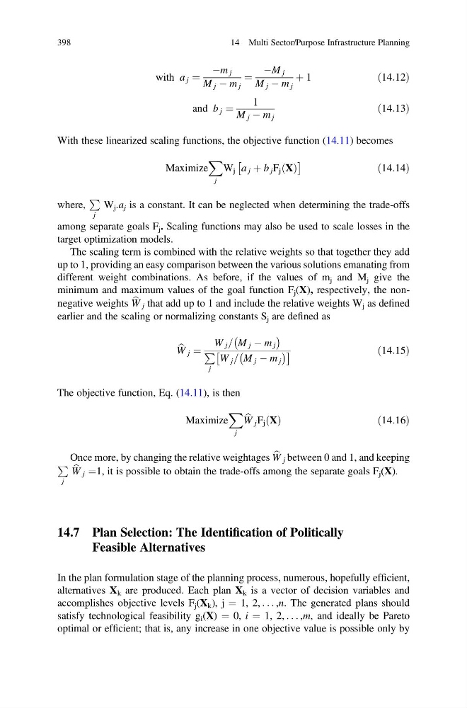
with a j ¼
Àm j
M j À m j
¼
ÀM j
M j À m j
þ 1
ð14:12Þ
and b j ¼
1
M j À m j
ð14:13Þ
With these linearized scaling functions, the objective function (14.11) becomes
Maximize
X
j
W j a j þ b j F j X
ð Þ
Â
Ã
ð14:14Þ
where,
P
j
W j .a j is a constant. It can be neglected when determining the trade-offs
among separate goals F j . Scaling functions may also be used to scale losses in the
target optimization models.
The scaling term is combined with the relative weights so that together they add
up to 1, providing an easy comparison between the various solutions emanating from
different weight combinations. As before, if the values of m j and M j give the
minimum and maximum values of the goal function F j (X), respectively, the nonnegative weights b
W j that add up to 1 and include the relative weights W j as defined
earlier and the scaling or normalizing constants S j are defined as
b
W j ¼
W j = M j À m j
À
Á
P
j
W j = M j À m j
À
Á
Â
Ã
ð14:15Þ
The objective function, Eq. (14.11), is then
Maximize
X
j
b
W j F j X
ð Þ
ð14:16Þ
Once more, by changing the relative weightages b
W j between 0 and 1, and keeping
P
j
b
W j ¼1, it is possible to obtain the trade-offs among the separate goals F j (X).
14.7 Plan Selection: The Identification of Politically
Feasible Alternatives
In the plan formulation stage of the planning process, numerous, hopefully efficient,
alternatives X k are produced. Each plan X k is a vector of decision variables and
accomplishes objective levels F j (X k ), j ¼ 1, 2, . . . ,n. The generated plans should
satisfy technological feasibility g i (X) ¼ 0, i ¼ 1, 2, . . . ,m, and ideally be Pareto
optimal or efficient; that is, any increase in one objective value is possible only by
398
14 Multi Sector/Purpose Infrastructure Planning
Àm j
M j À m j
¼
ÀM j
M j À m j
þ 1
ð14:12Þ
and b j ¼
1
M j À m j
ð14:13Þ
With these linearized scaling functions, the objective function (14.11) becomes
Maximize
X
j
W j a j þ b j F j X
ð Þ
Â
Ã
ð14:14Þ
where,
P
j
W j .a j is a constant. It can be neglected when determining the trade-offs
among separate goals F j . Scaling functions may also be used to scale losses in the
target optimization models.
The scaling term is combined with the relative weights so that together they add
up to 1, providing an easy comparison between the various solutions emanating from
different weight combinations. As before, if the values of m j and M j give the
minimum and maximum values of the goal function F j (X), respectively, the nonnegative weights b
W j that add up to 1 and include the relative weights W j as defined
earlier and the scaling or normalizing constants S j are defined as
b
W j ¼
W j = M j À m j
À
Á
P
j
W j = M j À m j
À
Á
Â
Ã
ð14:15Þ
The objective function, Eq. (14.11), is then
Maximize
X
j
b
W j F j X
ð Þ
ð14:16Þ
Once more, by changing the relative weightages b
W j between 0 and 1, and keeping
P
j
b
W j ¼1, it is possible to obtain the trade-offs among the separate goals F j (X).
14.7 Plan Selection: The Identification of Politically
Feasible Alternatives
In the plan formulation stage of the planning process, numerous, hopefully efficient,
alternatives X k are produced. Each plan X k is a vector of decision variables and
accomplishes objective levels F j (X k ), j ¼ 1, 2, . . . ,n. The generated plans should
satisfy technological feasibility g i (X) ¼ 0, i ¼ 1, 2, . . . ,m, and ideally be Pareto
optimal or efficient; that is, any increase in one objective value is possible only by
398
14 Multi Sector/Purpose Infrastructure Planning