

Thus, in Fig. 14.3, the parts ABC and DE of the feasibility frontier are convex. When
parts of the feasible boundary curve are not convex (e.g., curve CD), or if a portion is
convex but contains inferior points (e.g., curve AB), maximizing the various
weighted sums of individual goals/objectives will not produce all points on the
boundary curve. In such cases, the feasible boundary curve can be obtained by
limiting the values of some of the goals while maximizing the weighted combinations of the others.
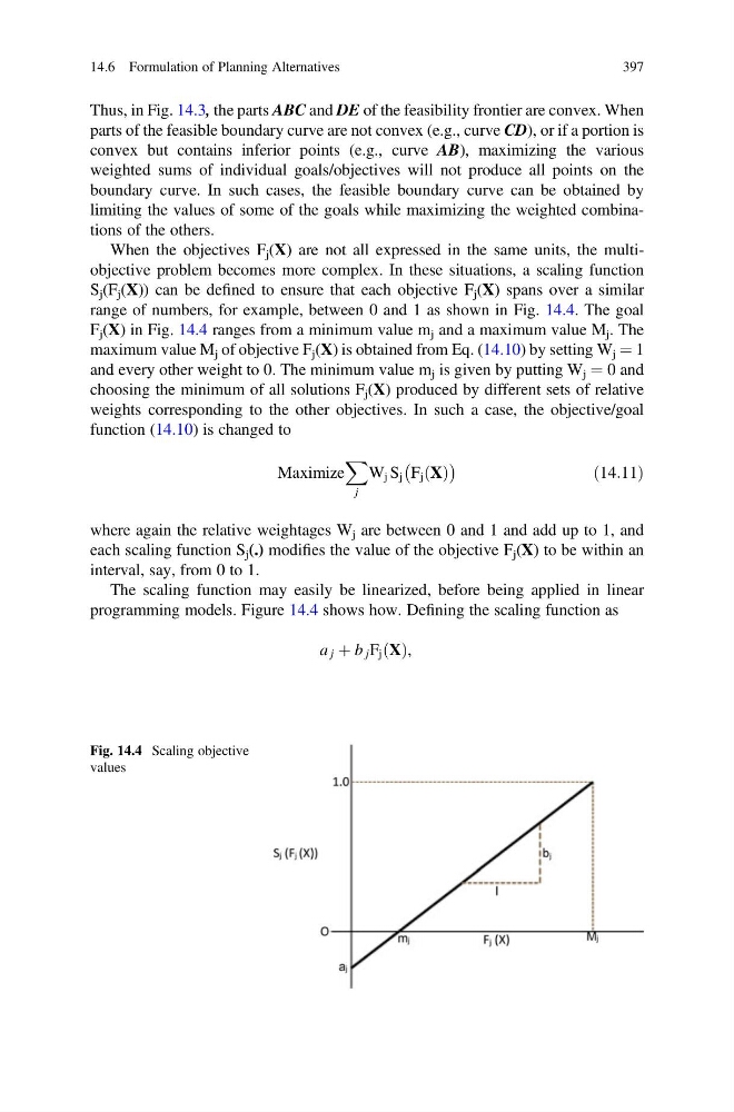
When the objectives F j (X) are not all expressed in the same units, the multiobjective problem becomes more complex. In these situations, a scaling function
S j (F j (X)) can be defined to ensure that each objective F j (X) spans over a similar
range of numbers, for example, between 0 and 1 as shown in Fig. 14.4. The goal
F j (X) in Fig. 14.4 ranges from a minimum value m j and a maximum value M j . The
maximum value M j of objective F j (X) is obtained from Eq. (14.10) by setting W j ¼ 1
and every other weight to 0. The minimum value m j is given by putting W j ¼ 0 and
choosing the minimum of all solutions F j (X) produced by different sets of relative
weights corresponding to the other objectives. In such a case, the objective/goal
function (14.10) is changed to
Maximize
X
j
W j S j F j X
ð Þ
À
Á
ð14:11Þ
where again the relative weightages W j are between 0 and 1 and add up to 1, and
each scaling function S j (.) modifies the value of the objective F j (X) to be within an
interval, say, from 0 to 1.
The scaling function may easily be linearized, before being applied in linear
programming models. Figure 14.4 shows how. Defining the scaling function as
a j þ b j F j X
ð Þ,
Fig. 14.4 Scaling objective
values
14.6 Formulation of Planning Alternatives
397
parts of the feasible boundary curve are not convex (e.g., curve CD), or if a portion is
convex but contains inferior points (e.g., curve AB), maximizing the various
weighted sums of individual goals/objectives will not produce all points on the
boundary curve. In such cases, the feasible boundary curve can be obtained by
limiting the values of some of the goals while maximizing the weighted combinations of the others.
When the objectives F j (X) are not all expressed in the same units, the multiobjective problem becomes more complex. In these situations, a scaling function
S j (F j (X)) can be defined to ensure that each objective F j (X) spans over a similar
range of numbers, for example, between 0 and 1 as shown in Fig. 14.4. The goal
F j (X) in Fig. 14.4 ranges from a minimum value m j and a maximum value M j . The
maximum value M j of objective F j (X) is obtained from Eq. (14.10) by setting W j ¼ 1
and every other weight to 0. The minimum value m j is given by putting W j ¼ 0 and
choosing the minimum of all solutions F j (X) produced by different sets of relative
weights corresponding to the other objectives. In such a case, the objective/goal
function (14.10) is changed to
Maximize
X
j
W j S j F j X
ð Þ
À
Á
ð14:11Þ
where again the relative weightages W j are between 0 and 1 and add up to 1, and
each scaling function S j (.) modifies the value of the objective F j (X) to be within an
interval, say, from 0 to 1.
The scaling function may easily be linearized, before being applied in linear
programming models. Figure 14.4 shows how. Defining the scaling function as
a j þ b j F j X
ð Þ,
Fig. 14.4 Scaling objective
values
14.6 Formulation of Planning Alternatives
397