

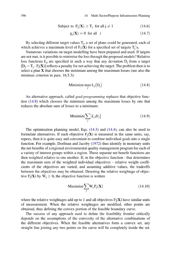
Subject to F j X
ð Þ ! T j for all j 6 ¼ 1
ð14:6Þ
g i X
ð Þ ¼ 0 for all i
ð14:7Þ
By selecting different target values T j , a set of plans could be generated, each of
which achieves a maximum level of F 1 (X) for a specified set of targets T j ’s.
Numerous variations on target modelling have been prepared and used. If targets
are not met, is it possible to minimise the loss through the proposed models? Relative
loss functions L j are specified in such a way that any deviation D j from a target
[D j ¼ T j - F j (X)] reflects a penalty for not achieving the target. The problem then is to
select a plan X that chooses the minimum among the maximum losses (see also the
minimax criterion in para. 16.5.3):
Minimize max
j
L j D j
À Á
ð14:8Þ
An alternative approach, called goal-programming replaces that objective function (14.8) which chooses the minimum among the maximum losses by one that
reduces the absolute sum of losses to a minimum:
Minimize
X
j
L j D j
ð14:9Þ
The optimization planning model, Eqs. (14.3) and (14.4), can also be used to
formulate alternatives. If each objective F j (X) is measured in the same units, say,
rupees, then it is quite easy and convenient to combine individual goals into a single
function. For example, Dorfman and Jacoby (1972) thus identify in monetary units
the net benefits of a regional environmental quality management program for each of
a variety of interest groups within a region. These separate net benefit functions are
then weighted relative to one another. If, in the objective function - that determines
the maximum sum of the weighted individual objectives – relative weight coefficients of the objectives are varied, and assuming additive values, the tradeoffs
between the objectives may be obtained. Denoting the relative weightage of objective F j (X) by W j ! 0, the objective function is written
Maximize
X
j
W j F j X
ð Þ
ð14:10Þ
where the relative weightages add up to 1 and all objectives F j (X) have similar units
of measurement. When the relative weightages are modified, other points are
obtained, thus defining the convex portion of the feasible boundary curve.
The success of any approach used to define the feasibility frontier critically
depends on the assumptions of the convexity of the alternative combinations of
the different objectives. When the feasible alternatives form a convex set, any
straight line joining any two points on the curve will lie completely inside the set.
396
14 Multi Sector/Purpose Infrastructure Planning
ð Þ ! T j for all j 6 ¼ 1
ð14:6Þ
g i X
ð Þ ¼ 0 for all i
ð14:7Þ
By selecting different target values T j , a set of plans could be generated, each of
which achieves a maximum level of F 1 (X) for a specified set of targets T j ’s.
Numerous variations on target modelling have been prepared and used. If targets
are not met, is it possible to minimise the loss through the proposed models? Relative
loss functions L j are specified in such a way that any deviation D j from a target
[D j ¼ T j - F j (X)] reflects a penalty for not achieving the target. The problem then is to
select a plan X that chooses the minimum among the maximum losses (see also the
minimax criterion in para. 16.5.3):
Minimize max
j
L j D j
À Á
ð14:8Þ
An alternative approach, called goal-programming replaces that objective function (14.8) which chooses the minimum among the maximum losses by one that
reduces the absolute sum of losses to a minimum:
Minimize
X
j
L j D j
ð14:9Þ
The optimization planning model, Eqs. (14.3) and (14.4), can also be used to
formulate alternatives. If each objective F j (X) is measured in the same units, say,
rupees, then it is quite easy and convenient to combine individual goals into a single
function. For example, Dorfman and Jacoby (1972) thus identify in monetary units
the net benefits of a regional environmental quality management program for each of
a variety of interest groups within a region. These separate net benefit functions are
then weighted relative to one another. If, in the objective function - that determines
the maximum sum of the weighted individual objectives – relative weight coefficients of the objectives are varied, and assuming additive values, the tradeoffs
between the objectives may be obtained. Denoting the relative weightage of objective F j (X) by W j ! 0, the objective function is written
Maximize
X
j
W j F j X
ð Þ
ð14:10Þ
where the relative weightages add up to 1 and all objectives F j (X) have similar units
of measurement. When the relative weightages are modified, other points are
obtained, thus defining the convex portion of the feasible boundary curve.
The success of any approach used to define the feasibility frontier critically
depends on the assumptions of the convexity of the alternative combinations of
the different objectives. When the feasible alternatives form a convex set, any
straight line joining any two points on the curve will lie completely inside the set.
396
14 Multi Sector/Purpose Infrastructure Planning