

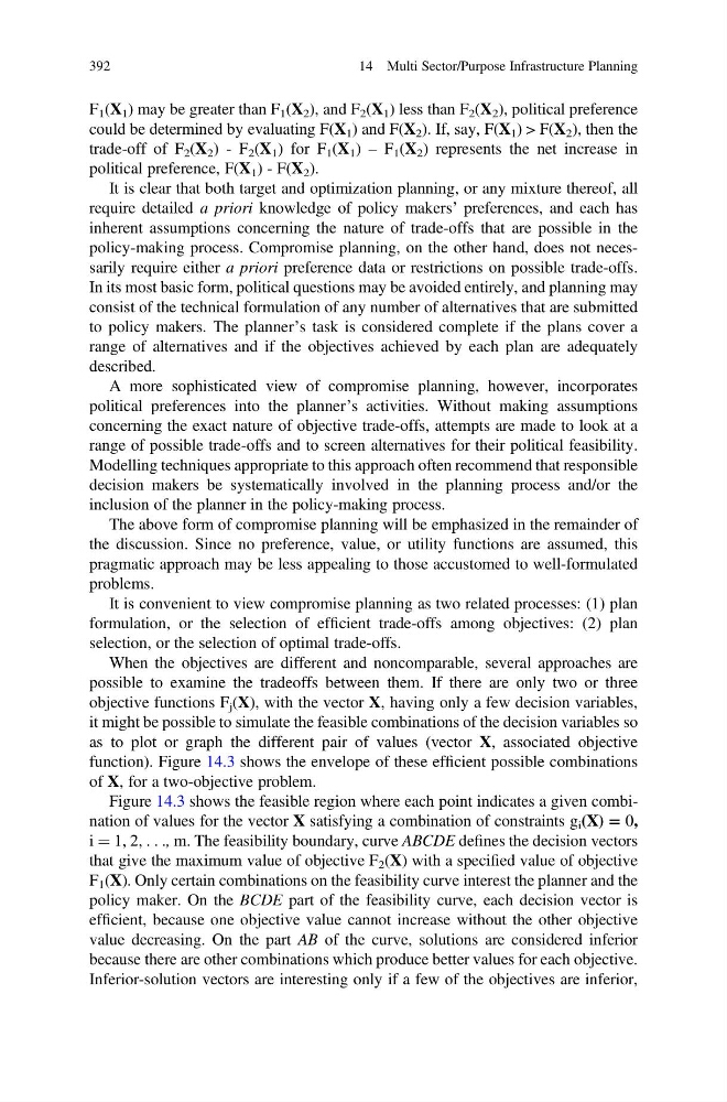
F 1 (X 1 ) may be greater than F 1 (X 2 ), and F 2 (X 1 ) less than F 2 (X 2 ), political preference
could be determined by evaluating F(X 1 ) and F(X 2 ). If, say, F(X 1 ) > F(X 2 ), then the
trade-off of F 2 (X 2 ) - F 2 (X 1 ) for F 1 (X 1 ) – F 1 (X 2 ) represents the net increase in
political preference, F(X 1 ) - F(X 2 ).
It is clear that both target and optimization planning, or any mixture thereof, all
require detailed a priori knowledge of policy makers’ preferences, and each has
inherent assumptions concerning the nature of trade-offs that are possible in the
policy-making process. Compromise planning, on the other hand, does not necessarily require either a priori preference data or restrictions on possible trade-offs.
In its most basic form, political questions may be avoided entirely, and planning may
consist of the technical formulation of any number of alternatives that are submitted
to policy makers. The planner’s task is considered complete if the plans cover a
range of alternatives and if the objectives achieved by each plan are adequately
described.
A more sophisticated view of compromise planning, however, incorporates
political preferences into the planner’s activities. Without making assumptions
concerning the exact nature of objective trade-offs, attempts are made to look at a
range of possible trade-offs and to screen alternatives for their political feasibility.
Modelling techniques appropriate to this approach often recommend that responsible
decision makers be systematically involved in the planning process and/or the
inclusion of the planner in the policy-making process.
The above form of compromise planning will be emphasized in the remainder of
the discussion. Since no preference, value, or utility functions are assumed, this
pragmatic approach may be less appealing to those accustomed to well-formulated
problems.
It is convenient to view compromise planning as two related processes: (1) plan
formulation, or the selection of efficient trade-offs among objectives: (2) plan
selection, or the selection of optimal trade-offs.
When the objectives are different and noncomparable, several approaches are
possible to examine the tradeoffs between them. If there are only two or three
objective functions F j (X), with the vector X, having only a few decision variables,
it might be possible to simulate the feasible combinations of the decision variables so
as to plot or graph the different pair of values (vector X, associated objective
function). Figure 14.3 shows the envelope of these efficient possible combinations
of X, for a two-objective problem.
Figure 14.3 shows the feasible region where each point indicates a given combination of values for the vector X satisfying a combination of constraints g i (X) = 0,
i ¼ 1, 2, . . ., m. The feasibility boundary, curve ABCDE defines the decision vectors
that give the maximum value of objective F 2 (X) with a specified value of objective
F 1 (X). Only certain combinations on the feasibility curve interest the planner and the
policy maker. On the BCDE part of the feasibility curve, each decision vector is
efficient, because one objective value cannot increase without the other objective
value decreasing. On the part AB of the curve, solutions are considered inferior
because there are other combinations which produce better values for each objective.
Inferior-solution vectors are interesting only if a few of the objectives are inferior,
392
14 Multi Sector/Purpose Infrastructure Planning
could be determined by evaluating F(X 1 ) and F(X 2 ). If, say, F(X 1 ) > F(X 2 ), then the
trade-off of F 2 (X 2 ) - F 2 (X 1 ) for F 1 (X 1 ) – F 1 (X 2 ) represents the net increase in
political preference, F(X 1 ) - F(X 2 ).
It is clear that both target and optimization planning, or any mixture thereof, all
require detailed a priori knowledge of policy makers’ preferences, and each has
inherent assumptions concerning the nature of trade-offs that are possible in the
policy-making process. Compromise planning, on the other hand, does not necessarily require either a priori preference data or restrictions on possible trade-offs.
In its most basic form, political questions may be avoided entirely, and planning may
consist of the technical formulation of any number of alternatives that are submitted
to policy makers. The planner’s task is considered complete if the plans cover a
range of alternatives and if the objectives achieved by each plan are adequately
described.
A more sophisticated view of compromise planning, however, incorporates
political preferences into the planner’s activities. Without making assumptions
concerning the exact nature of objective trade-offs, attempts are made to look at a
range of possible trade-offs and to screen alternatives for their political feasibility.
Modelling techniques appropriate to this approach often recommend that responsible
decision makers be systematically involved in the planning process and/or the
inclusion of the planner in the policy-making process.
The above form of compromise planning will be emphasized in the remainder of
the discussion. Since no preference, value, or utility functions are assumed, this
pragmatic approach may be less appealing to those accustomed to well-formulated
problems.
It is convenient to view compromise planning as two related processes: (1) plan
formulation, or the selection of efficient trade-offs among objectives: (2) plan
selection, or the selection of optimal trade-offs.
When the objectives are different and noncomparable, several approaches are
possible to examine the tradeoffs between them. If there are only two or three
objective functions F j (X), with the vector X, having only a few decision variables,
it might be possible to simulate the feasible combinations of the decision variables so
as to plot or graph the different pair of values (vector X, associated objective
function). Figure 14.3 shows the envelope of these efficient possible combinations
of X, for a two-objective problem.
Figure 14.3 shows the feasible region where each point indicates a given combination of values for the vector X satisfying a combination of constraints g i (X) = 0,
i ¼ 1, 2, . . ., m. The feasibility boundary, curve ABCDE defines the decision vectors
that give the maximum value of objective F 2 (X) with a specified value of objective
F 1 (X). Only certain combinations on the feasibility curve interest the planner and the
policy maker. On the BCDE part of the feasibility curve, each decision vector is
efficient, because one objective value cannot increase without the other objective
value decreasing. On the part AB of the curve, solutions are considered inferior
because there are other combinations which produce better values for each objective.
Inferior-solution vectors are interesting only if a few of the objectives are inferior,
392
14 Multi Sector/Purpose Infrastructure Planning