

i.e., if they have to be minimized (the negative-slope of the decision maker‘s
indifference curve would point to such a situation). Only the efficient superior
solutions need be taken into account, if all objectives are superior.
Using simulation models to define the feasibility curve and the corresponding
trade-offs between the efficient decision vectors becomes less easy with an increasing number of parameters and objectives. When there are more than three objectives,
it becomes impossible to show the trade-offs between objectives F j (X), graphically.
Therefore, the estimation of feasible and efficient decision vectors X is often carried
out using optimization techniques.
It may be useful to observe that different models - using different assumptions - of
the same problem could produce different feasibility boundary curves. Simplifications, often dictated by algorithmic, computer, available data, or budget limitations,
provide the main reasons for possible uncertainties associated with the feasibility
frontier obtained. It is also possible that what appears feasible ex ante is not feasible
ex post, or vice versa, regardless of the model used to define feasibility. However, it
is assumed, here, that the planning process does result in a reasonably accurate and
well delineated feasibility frontier and, thus, a finite set of efficient alternatives from
which a choice can be made.
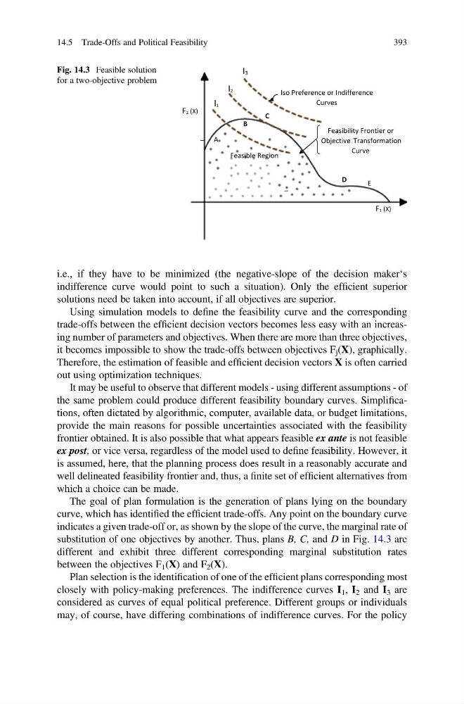
The goal of plan formulation is the generation of plans lying on the boundary
curve, which has identified the efficient trade-offs. Any point on the boundary curve
indicates a given trade-off or, as shown by the slope of the curve, the marginal rate of
substitution of one objectives by another. Thus, plans B, C, and D in Fig. 14.3 are
different and exhibit three different corresponding marginal substitution rates
between the objectives F 1 (X) and F 2 (X).
Plan selection is the identification of one of the efficient plans corresponding most
closely with policy-making preferences. The indifference curves I 1 , I 2 and I 3 are
considered as curves of equal political preference. Different groups or individuals
may, of course, have differing combinations of indifference curves. For the policy
I1
I2
I3
A
B
C
Iso Preference or Indifference
Curves
F2 (X)
F1 (X)
Feasible Region
Feasibility Frontier or
Objective Transformation
Curve
D
E
Fig. 14.3 Feasible solution
for a two-objective problem
14.5 Trade-Offs and Political Feasibility
393
indifference curve would point to such a situation). Only the efficient superior
solutions need be taken into account, if all objectives are superior.
Using simulation models to define the feasibility curve and the corresponding
trade-offs between the efficient decision vectors becomes less easy with an increasing number of parameters and objectives. When there are more than three objectives,
it becomes impossible to show the trade-offs between objectives F j (X), graphically.
Therefore, the estimation of feasible and efficient decision vectors X is often carried
out using optimization techniques.
It may be useful to observe that different models - using different assumptions - of
the same problem could produce different feasibility boundary curves. Simplifications, often dictated by algorithmic, computer, available data, or budget limitations,
provide the main reasons for possible uncertainties associated with the feasibility
frontier obtained. It is also possible that what appears feasible ex ante is not feasible
ex post, or vice versa, regardless of the model used to define feasibility. However, it
is assumed, here, that the planning process does result in a reasonably accurate and
well delineated feasibility frontier and, thus, a finite set of efficient alternatives from
which a choice can be made.
The goal of plan formulation is the generation of plans lying on the boundary
curve, which has identified the efficient trade-offs. Any point on the boundary curve
indicates a given trade-off or, as shown by the slope of the curve, the marginal rate of
substitution of one objectives by another. Thus, plans B, C, and D in Fig. 14.3 are
different and exhibit three different corresponding marginal substitution rates
between the objectives F 1 (X) and F 2 (X).
Plan selection is the identification of one of the efficient plans corresponding most
closely with policy-making preferences. The indifference curves I 1 , I 2 and I 3 are
considered as curves of equal political preference. Different groups or individuals
may, of course, have differing combinations of indifference curves. For the policy
I1
I2
I3
A
B
C
Iso Preference or Indifference
Curves
F2 (X)
F1 (X)
Feasible Region
Feasibility Frontier or
Objective Transformation
Curve
D
E
Fig. 14.3 Feasible solution
for a two-objective problem
14.5 Trade-Offs and Political Feasibility
393