

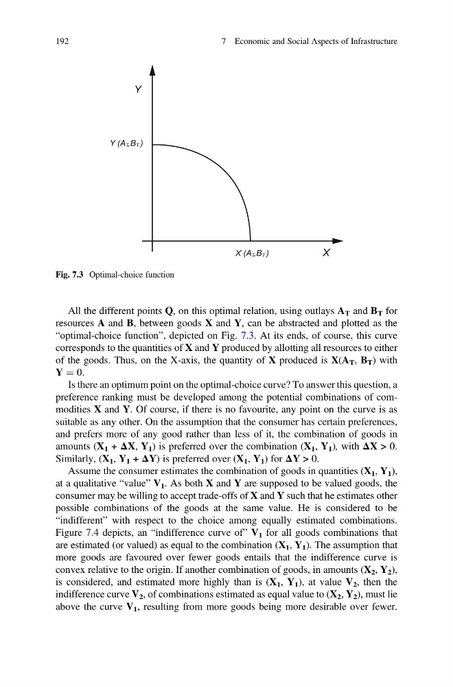
All the different points Q, on this optimal relation, using outlays A T and B T for
resources A and B, between goods X and Y, can be abstracted and plotted as the
“optimal-choice function”, depicted on Fig. 7.3. At its ends, of course, this curve
corresponds to the quantities of X and Y produced by allotting all resources to either
of the goods. Thus, on the X-axis, the quantity of X produced is X(A T , B T ) with
Y ¼ 0.
Is there an optimum point on the optimal-choice curve? To answer this question, a
preference ranking must be developed among the potential combinations of commodities X and Y. Of course, if there is no favourite, any point on the curve is as
suitable as any other. On the assumption that the consumer has certain preferences,
and prefers more of any good rather than less of it, the combination of goods in
amounts (X 1 + ΔX, Y 1 ) is preferred over the combination (X 1 , Y 1 ), with ΔX > 0.
Similarly, (X 1 , Y 1 + ΔY) is preferred over (X 1 , Y 1 ) for ΔY > 0.
Assume the consumer estimates the combination of goods in quantities (X 1 , Y 1 ),
at a qualitative “value” V 1 . As both X and Y are supposed to be valued goods, the
consumer may be willing to accept trade-offs of X and Y such that he estimates other
possible combinations of the goods at the same value. He is considered to be
“indifferent” with respect to the choice among equally estimated combinations.
Figure 7.4 depicts, an “indifference curve of” V 1 for all goods combinations that
are estimated (or valued) as equal to the combination (X 1 , Y 1 ). The assumption that
more goods are favoured over fewer goods entails that the indifference curve is
convex relative to the origin. If another combination of goods, in amounts (X 2 , Y 2 ),
is considered, and estimated more highly than is (X 1 , Y 1 ), at value V 2 , then the
indifference curve V 2 , of combinations estimated as equal value to (X 2 , Y 2 ), must lie
above the curve V 1 , resulting from more goods being more desirable over fewer.
X
Y
Y (A ,B )
T T
X (A ,B )
T T
Fig. 7.3 Optimal-choice function
192
7 Economic and Social Aspects of Infrastructure
resources A and B, between goods X and Y, can be abstracted and plotted as the
“optimal-choice function”, depicted on Fig. 7.3. At its ends, of course, this curve
corresponds to the quantities of X and Y produced by allotting all resources to either
of the goods. Thus, on the X-axis, the quantity of X produced is X(A T , B T ) with
Y ¼ 0.
Is there an optimum point on the optimal-choice curve? To answer this question, a
preference ranking must be developed among the potential combinations of commodities X and Y. Of course, if there is no favourite, any point on the curve is as
suitable as any other. On the assumption that the consumer has certain preferences,
and prefers more of any good rather than less of it, the combination of goods in
amounts (X 1 + ΔX, Y 1 ) is preferred over the combination (X 1 , Y 1 ), with ΔX > 0.
Similarly, (X 1 , Y 1 + ΔY) is preferred over (X 1 , Y 1 ) for ΔY > 0.
Assume the consumer estimates the combination of goods in quantities (X 1 , Y 1 ),
at a qualitative “value” V 1 . As both X and Y are supposed to be valued goods, the
consumer may be willing to accept trade-offs of X and Y such that he estimates other
possible combinations of the goods at the same value. He is considered to be
“indifferent” with respect to the choice among equally estimated combinations.
Figure 7.4 depicts, an “indifference curve of” V 1 for all goods combinations that
are estimated (or valued) as equal to the combination (X 1 , Y 1 ). The assumption that
more goods are favoured over fewer goods entails that the indifference curve is
convex relative to the origin. If another combination of goods, in amounts (X 2 , Y 2 ),
is considered, and estimated more highly than is (X 1 , Y 1 ), at value V 2 , then the
indifference curve V 2 , of combinations estimated as equal value to (X 2 , Y 2 ), must lie
above the curve V 1 , resulting from more goods being more desirable over fewer.
X
Y
Y (A ,B )
T T
X (A ,B )
T T
Fig. 7.3 Optimal-choice function
192
7 Economic and Social Aspects of Infrastructure